6.041/6.431 Probability - The Science of Uncertainty and Data
Lecture 1 (September 10, 2018)
Probability Models
To specify such a model, it includes 2 steps:
- Sample space: describe possible outcomes of an experiment
- Probability laws: describe beliefs about the likelihood of outcomes (or assign a probability to outcomes)
Sample space
list of possible outcomes must be mutually exclusive, collectively exhaustive, and at the right granularity.
Probability laws
Probability axioms
Motivation: Assign individual probability to a single dot is a challenge (in the dart example, each dot has zero probability), so we assign a probability to the subset of the sample space.
- Nonnegativity: {\bf P}(A) \geq 0
- Normalization: {\bf P}(\Omega) = 1
- (Finite) Additivity: if A \cap B = \emptyset then {\bf P}(A \cup B) = {\bf P}(A) + {\bf P}(B) (need to be refined in future)
Consequences of axioms (properties of probability axioms)
- {\bf P}(A) \leq 1
- {\bf P}(\emptyset) = 0
- {\bf P}(A) + {\bf P}(A^c) = 1
- A, B, \text{and } C are disjoint: {\bf P}(A \cup B \cup C) = {\bf P}(A) + {\bf P}(B) + {\bf P}(C)
- A_1, \cdots A_k, are disjoint: {\bf P}(A_1 \cup \cdots, \cup A_k) = \sum_{i - 1}^k{\bf P}(A_i)
- If A \subset B, then {\bf P}(A) \leq {\bf P}(B)
- {\bf P}(A \cup B) = {\bf P}(A) + {\bf P}(B) - {\bf P}(A \cap B)
- {\bf P}(A \cup B \cup C) = {\bf P}(A) + {\bf P}(A^c \cap B) + {\bf P}(A^c \cap B^c \cap C)
- Union Bound: {\bf P}(A \cup B) \leq {\bf P}(A) + {\bf P}(B)
Probability calculation steps
- Specify the sample space
- Specify a probability law
- Identify an event of interest
- Calculate
Countable additivity
The 3rd probability axiom previously mentioned can be extended to countable set (all integers), which means that the element in the set can be arranged in a sequence. This is contrary to the concept of uncountable set (i.e. a dart board, 2D plane). So you need to distinguish the following concepts:
- discrete set (countable set)
- continuous set (uncountable set, impossible to arrange in a sequence)
- finite set
- infinite set (possible to be arranged in a sequence)
- discrete (countable) finite set (i.e. {1, 2, 3})
- discrete (countable) infinite set (i.e. all integers, all even integers, all old integers)
- continuous (uncountable) infinite set (i.e. \{x | 0 \leq x \leq 1\})
Example: Sample space \{1, 2, 3, \cdots\}, given {\bf P}(n) = \frac{1}{2^n}, n = 1, 2, \cdots. Check the against the probability axioms that \sum_{n = 1}^{\infty}{\bf P}(n) = 1. What about the probability {\bf P}(\text{outcome is even})? Using countable additivity axiom.
Countable Additivity Axiom (refined probability axiom)
Note
if A_1, A_2, A_3, \cdot is an infinite sequence of disjoint events, then {\bf P}(A_1 \cup A_2 \cup A_3 \cdots) = {\bf P}(A_1) + {\bf P}(A_2) + {\bf P}(A_3) + \cdots
To refine the 3rd probability axiom, additivity holds only for "countable" sequences of events. That means the additivity axiom must be a sequence, with finite or infinite elements.
Note the following contradiction, the additivity axiom can not be applied to continuous sample space.
A_1, A_2, A_3, \cdots are real coordinates, if you apply the additivity axiom, you will get:
which is contradicts. This is because "unit square" is not a countable set.
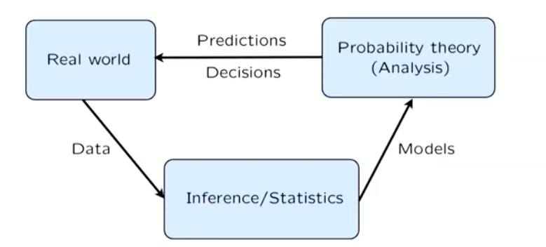
Interpretations of probability theory
-
frequency of events A?
- What is P(the president will be reelected)?
-
Probability is often interpreted as:
- Description of beliefs
- Betting preference
Lecture 2 Conditioning and Baye's rule
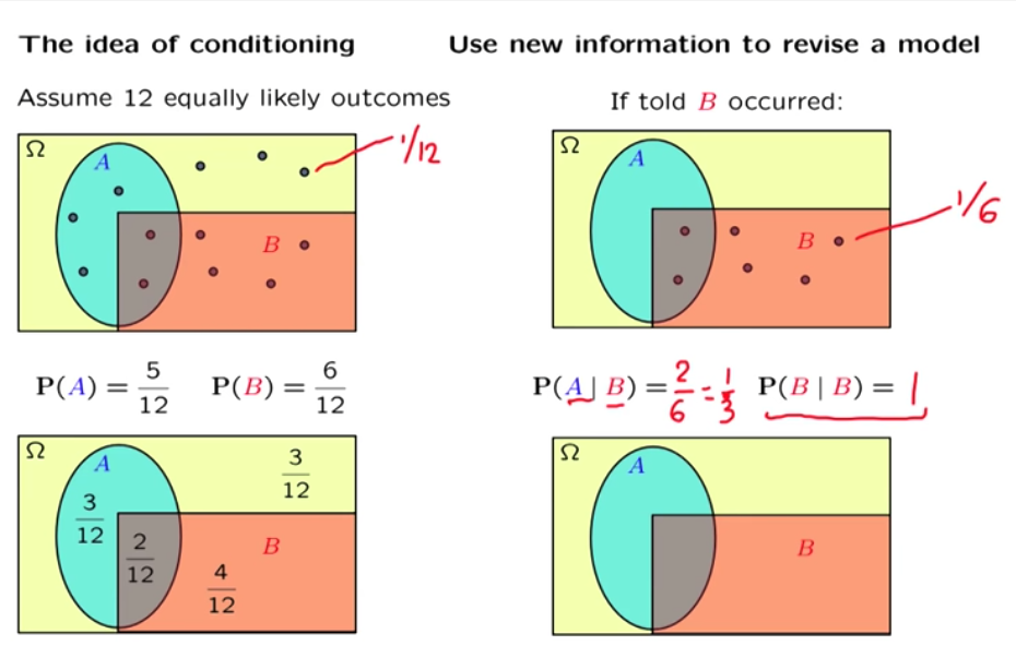
Conditional probability
use new information to review a model
Definition
{\bf P}(A|B) = "probability of A given that B occurred"
{\bf P}(A|B) = \frac{{\bf P}(A \cap B)}{{\bf P}(B)}, defined only when {\bf P}(B) > 0
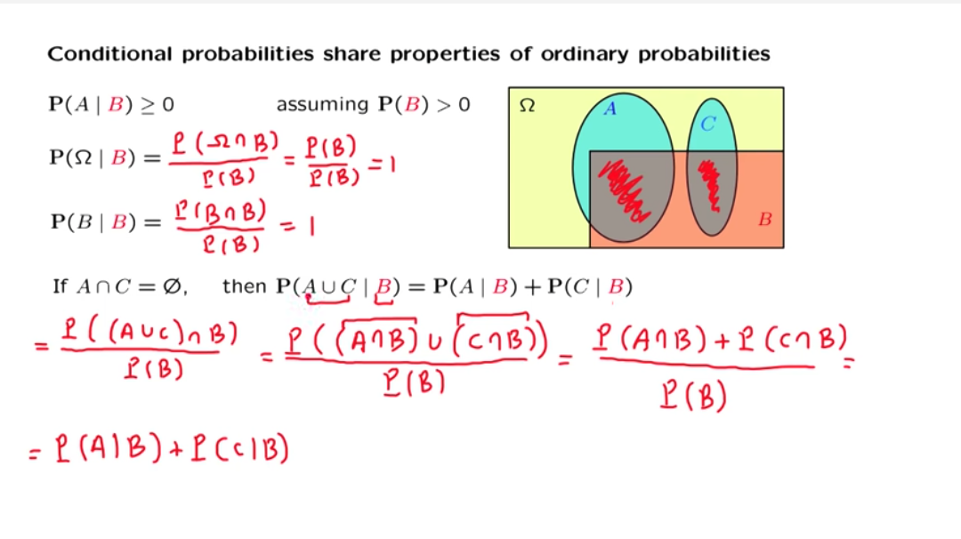
Conditional probability share properties of ordinary probabilities (finite and infinite countable additivity)
If A \cap C = \emptyset, then {\bf P}(A \cup C|B) = P(A|B) + {\bf P}(C|B)
Multiplication rule
{\bf P}(A \cap B) = {\bf P}(A){\bf P}(B|A) = {\bf P}(B){\bf P}(A|B)
{\bf P}(A \cap B \cap C) = {\bf P}(A){\bf P}(B|A){\bf P}(C|A \cap B)
It also applies to n events.
Total probability theorem (divide and conquer)
The settings:
- Partition of sample space into A_1, A_2, A_3,
- have {\bf P}(A_i) for every i
- have{\bf P}(B|A_i) for every i
{\bf P}(B) = \sum_{i} {\bf P}(A_i){\bf P}(B|A_i)
It also applies to infinite countable sets according to the countable additivity axiom.
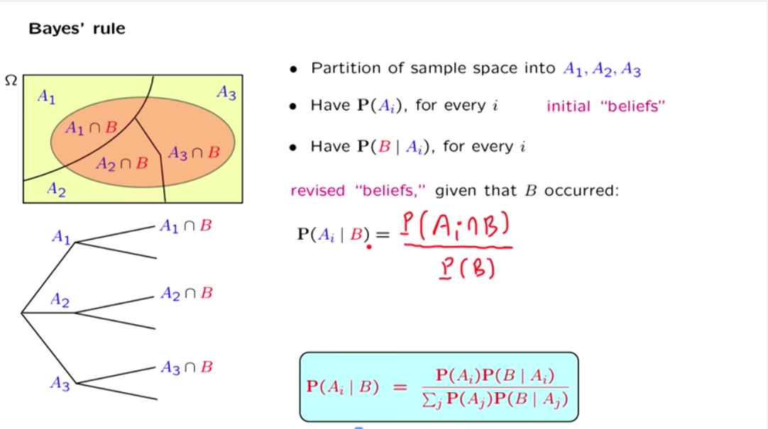
Baye's rule
The setting is the same as the total probability theorem.
- Partition of sample space into A_1, A_2, A_3,
- have {\bf P}(A_i) for every i (initial believes)
- have{\bf P}(B|A_i) for every i
revise "believe" given that B occurred:
{\bf P}(A_i|B) = \frac{{\bf P}(A_i \cap B)}{{\bf P}(B)}
It turns out that we can use multiplication rule to calculate the nominator and use the total probability rule to calculate the denominator, thusly
{\bf P}(A_i|B) = \frac{{\bf P}(A_i){\bf P}(B|A_i)}{\sum_j{\bf P}(A_j){\bf P}(B|A_i)}
Lecture 3 Independence
Independence of two events
Motivation
coin toss example: First toss is head or tail doesn't affect the probability of second toss is head.
Occurance of A privides no new information about B: {\bf P}(B|A) = {\bf P}(B).
Definition of independence
Formal definition
{\bf P}(A \cap B) = {\bf P}(A) \cdot {\bf P}(B)
- symmetric with respect to events.
- implies {\bf P}(A|B) = {\bf P}(A).
- Applies even if {\bf P}(A) = 0.
Distinction between disjoin and independence
Disjoin usually means dependent, because if one event happens we know the other event will not happen. 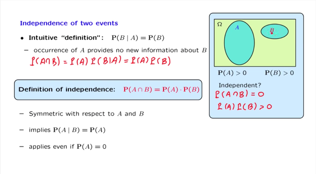
Independence of event complements
If A and B are independent, the A and B^c are independent.
If A and B are independent, the A^c and B^c are independent.
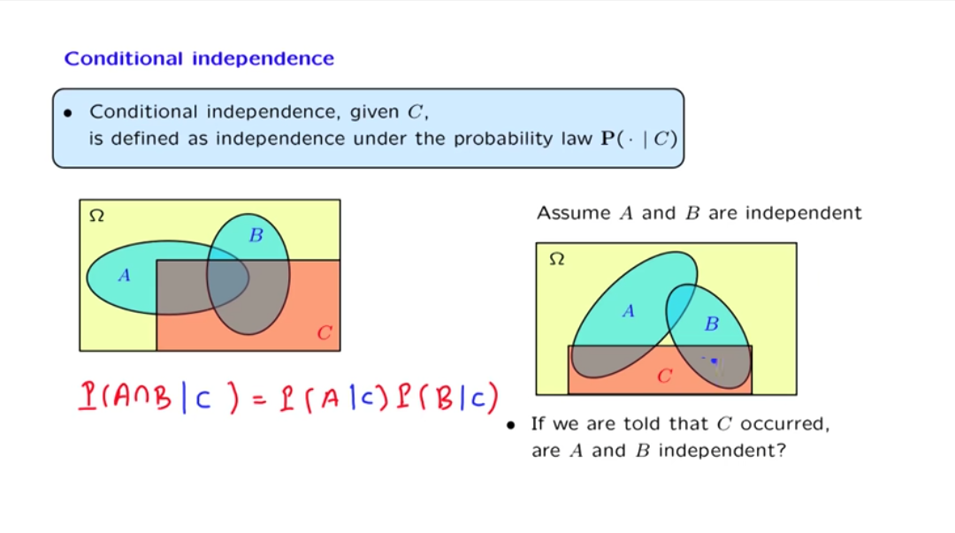
Conditioning independence
Ordinary independence properties also apply to conditional independence. But independence doesn't imply conditional independence.
Independence of a collection of events
Intuition "definition": Information on some of the events doesn't change probability related to the remaining events.
Formal definition
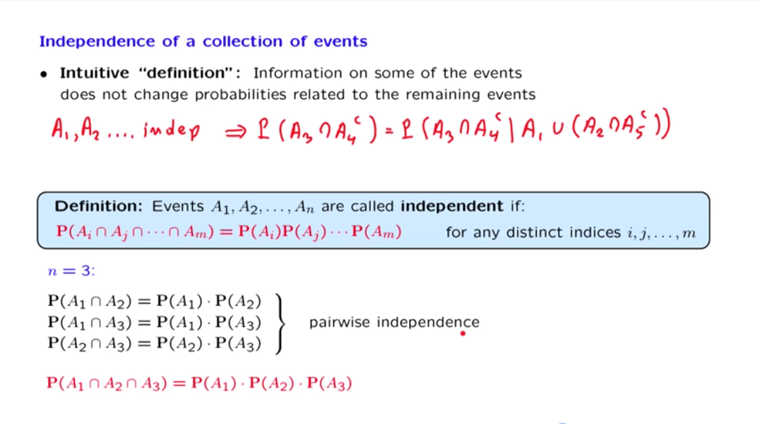
pairwise independence
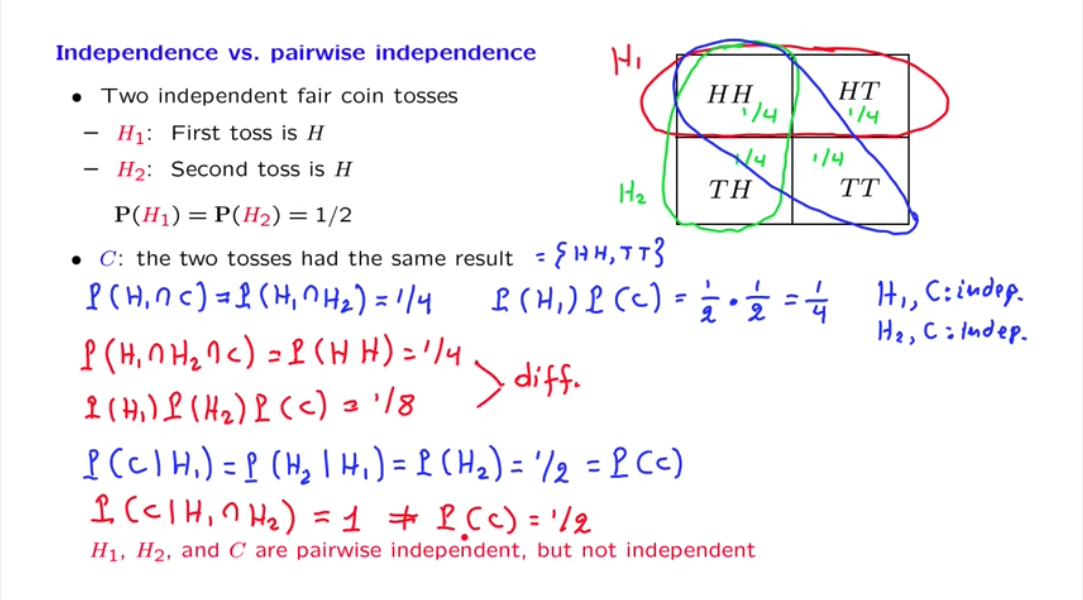
independence V.S. pairwise independence
Used two independence fair coin tosses as an example to show that pariwise independence isn't enough to show independence of collection of events.
Reliability
The king's sibling puzzle
Monty Hall problem
Lecture 4
Lecture 5
Definition of random variables
- A random variable ("r.v.") associates a value (a number) to every possible outcome.
- Mathematically, A function from sample space \Omega to the real numbers (discrete or continuous).
- We can have several random variables defined on the same sample space. (In Lecture 18, X_1, X_2, \cdots are independent random variables from the same distribution)
- A function of one or several random variables is also another random variable.
- A concrete example to understand the concept of a random variable is take a class of students, selecting students and measuring their body mass or height will give us the random variable W and H. The "Body mass index" is another random variable that is a function of the random variable W and H.
meaning of X + Y
random variable X+Y takes the value x+y, when X takes the value x, and Y takes the value y.
Probability mass function
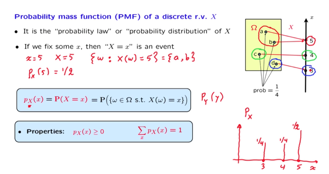
Bernoulli and indicator random variables
- Bernoulli random variable X: X = \begin{cases} 1, & \textrm{w.p. } p \\ 0, & \textrm{w.p. } 1-p \end{cases}
- models a trial that results in success/failure, heads/tails, etc.
- indicator random variables of event A: I_A = 1 if A occurs.
- connection between events and random variables. P(A) = P(I_A = 1) = P_{I_A}(1),
- P(A): probability of event A happens
- P(I_A = 1): probablistic notition of indication R.V. when I_A equal to 1
- P_{I_A}(1): PMF notation.
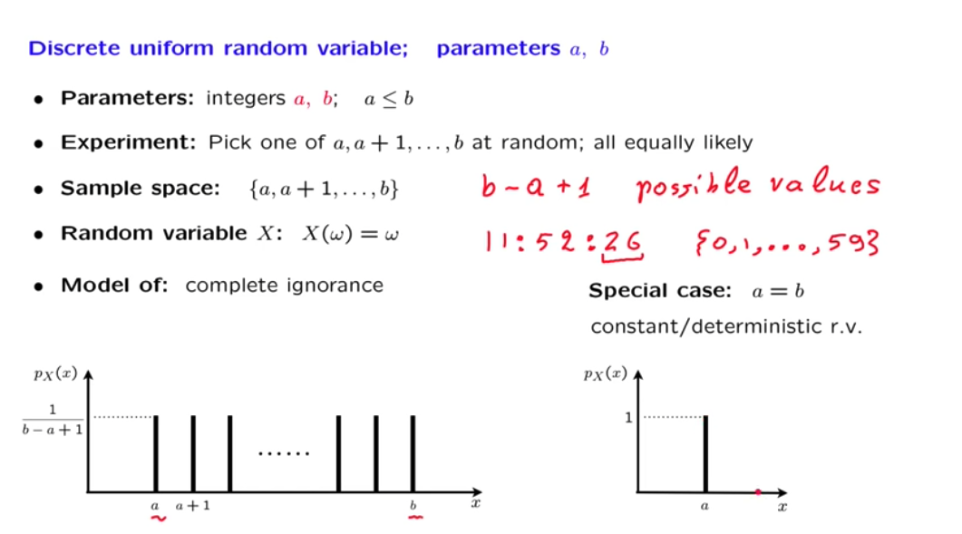
Discrete uniform random variables
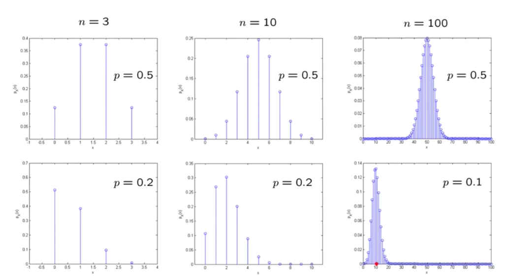
Binomial random variables
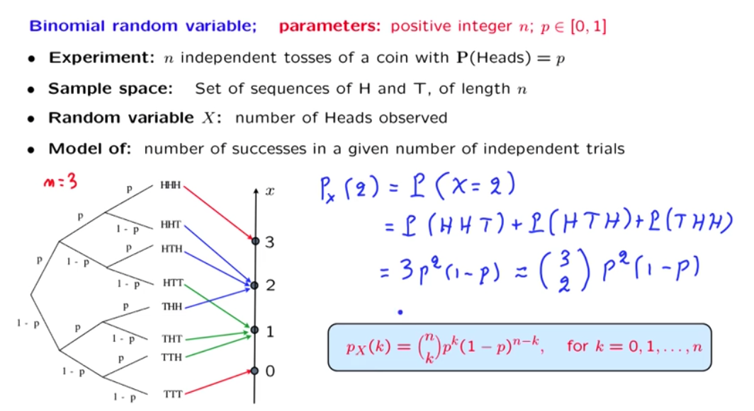
Experiment: toss a biased coin (P(\textrm{Head})=p) n times and observe the result (number of heads)
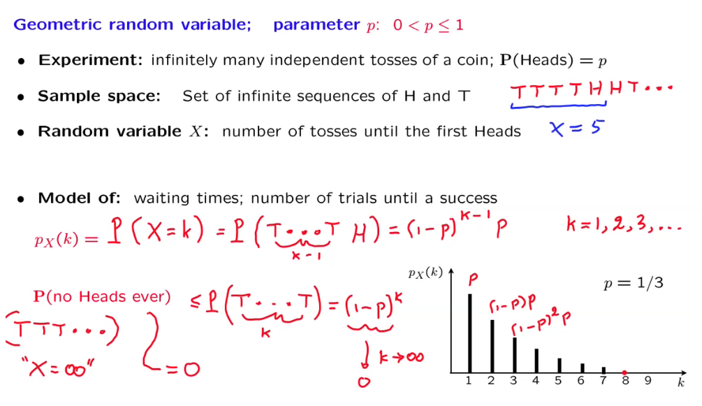
Geometric random variables
Expectation
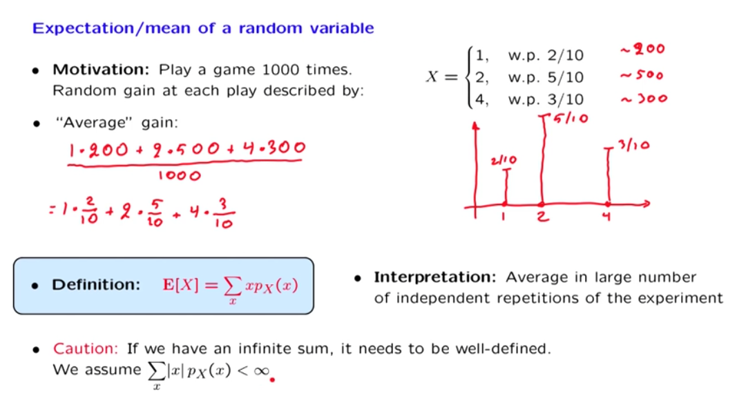
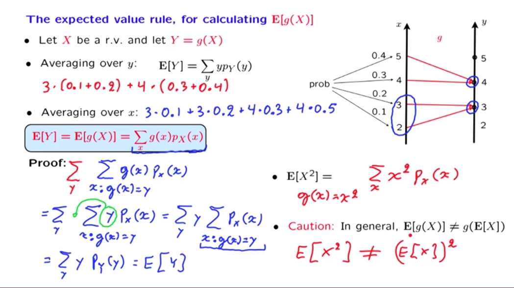
The expected value rule
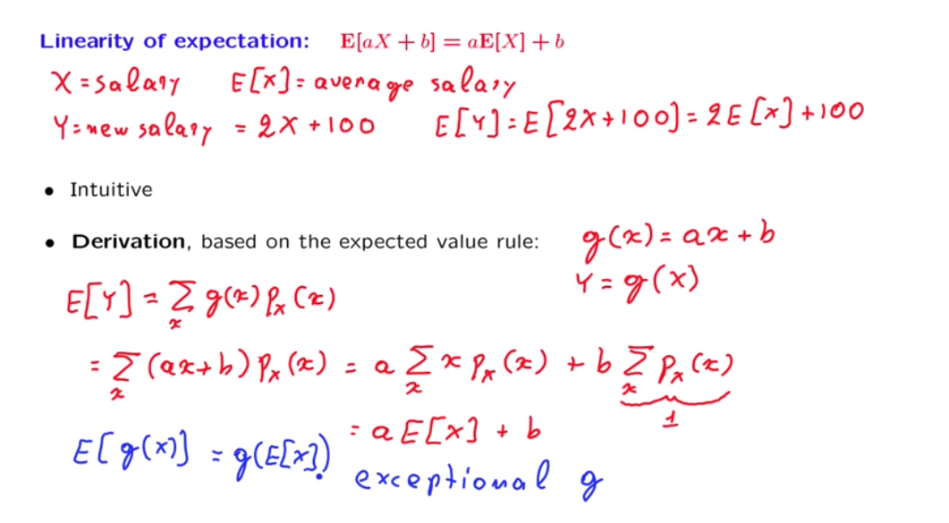
Linearity of expectations
Lecture 6
Lecture 7
Independence, variances, and binomial variance
Lecture 8
Exponential random variables
-
PDF: f_{X}(x) = \begin{cases} \lambda e^{-\lambda x}, & x \ge 0 \\ 0, & x < 0 \end{cases}
-
Probability of greater than a,
- Expectation of exponential random variable
{\bf E}\big[X\big] = \displaystyle \int_0^{\infty} x \cdot \lambda e^{-\lambda x} dx = 1/\lambda
- Second moment of an exponential random variable
{\bf E}\big[X^2 \big] = \displaystyle \int_0^{\infty} x^2 \cdot \lambda e^{-\lambda x} dx = 2/\lambda^2
- Variance of an exponential random variable
\textbf{Var}(X) = {\bf E}\big[X^2 \big] - \Big({\bf E}\big[X\big]\Big)^2 = 1/\lambda^2
Lecture 9
Conditioning a continuous random variable on an event
Memorylessness of the exponential PDF
Total probability and expectation theorems
Lecture 10
Total probability and total expectation theorems
Follows from the discrete cases:
| Rules | Discrete | continous |
|---|---|---|
| Total probability | p_X(x) = \displaystyle \sum\limits_{y} p_Y(y)p_{X \mid Y}(x \mid y) | f_X(x) = \displaystyle \int_{-\infty}^{+\infty} f_Y(y) f_{X \mid Y}(x \mid y) dy |
| Conditional expectation | {\bf E}\big[X \mid Y = y \big] = \displaystyle \sum\limits_{x} x p_{X \mid Y}(x \mid y) | {\bf E}\big[X \mid Y = y \big] = \displaystyle {\int_{-\infty}^{+\infty}} x f_{X \mid Y}(x \mid y) dx |
| Total expectation | {\bf E}\big[X \big] = \displaystyle \sum\limits_{y} p_{Y}(y){\bf E} \big[X \mid Y = y \big] derivation hint: replace with the conditional expectatioin | {\bf E}\big[X \big] = \displaystyle {\int_{-\infty}^{+\infty}} f_{Y}(y){\bf E}\big[X \mid Y = y \big] dy derivation hint: replace with the conditional expectatioin |
| Expected value rule | {\bf E}\big[ g(X) \mid Y = y \big] = \displaystyle {\sum\limits_{x}} g(x) p_{X \mid Y}(x \mid y) | {\bf E}\big[ g(X) \mid Y = y \big] = \displaystyle {\int_{-\infty}^{+\infty}} g(x) f_{X \mid Y}(x \mid y) dx |
Solved problems (Lecture 8 - 10)
10 Buffon's needle and Monte Carlo Simulation
This problem is discussed in the text page 161, Example 3.11.
Lecture 11
Lecture 12
Covariance
- Definition: \textbf{cov}(X, Y) = {\bf E}\big[(X - {\bf E}[X]) (Y - {\bf E}[Y])\big]
- Covariance tell use whether two r.v.s tend to move together, both to low or both to high
- Two random variables X and Y are independent indicates: \textbf{cov}(X, Y) = 0, but the converse it not true.
Covariance properties
Lecture 13
The conditional expectation as a random variable {\bf E} \big[X \mid Y\big]
- Given a function h(x) = x^2 for all x, and a random variable X. what is h(X)?
- h(X) is a function of a random variable X. h(X) itself is a random variable that take value x^2 if X happens to take the value x. (you should really understand this statement, it is crucial to understand the concept of conditional expectatioin)
- For discrete case: {\bf E}\big[X \mid Y = y \big] = \displaystyle \sum\limits_{x} x p_{X \mid Y}(x \mid y), in which different vaule of y will give us the different value of conditional expectation of X. Then we can really treat {\bf E}\big[X \mid Y = y \big] as a function of y, noted as g(y).
- From the above reasoning, because Y is a random variable, g(Y) is also a reandom variable, that takes the value of g(y) = {\bf E}\big[X \mid Y = y \big] if Y happens to take the value y.
- g(Y) = {\bf E}\big[X \mid Y\big], is
- a function of Y
- a random variable
- has a distribution, mean, variance, etc.
The law of iterated expectations
By calculate {\bf E}\Big[{\bf E}\big[X \mid Y\big]\Big], we could abtain that it is equal to {\bf E}\big[X\big]
The conditional variance as a random variable \textbf{Var}(X \mid Y = y)
- definition: \textbf{Var}(X \mid Y = y) = {\bf E}\Big[\big(X - {\bf E}\big[X \mid Y = y \big]\big)^2\mid Y = y\Big]
- \textbf{Var}(X\mid Y) is also a random variable, it takes the value \textbf{Var}(X\mid y) when Y happens to take the value of y.
- Total variance rule: \textbf{Var}(X) = {\bf E}\Big[\textbf{Var}(X \mid Y)\Big] + \textbf{Var}\Big({\bf E}\big[X\mid Y\big]\Big)
Lecture 14 Introduction to Bayesian Inference
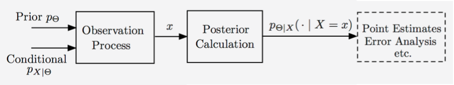
The Bayesian inference framework
Treat the unknown \Theta as a random variable. with prior p_{\Theta} or f_{\Theta}. With the observations X, using Bayes rule to obtain the posterior probability of \Theta, P_{\Theta|X}(\cdot|X=x). Once the posterior is available, the estimator can be obtained via maximize a posterioral probability (MAP) rule or leaset mean squares (LMS). The performance can be measured by "probability of error" or "mean squared error".
Conditional probability of error and total probability of error
- The conditional probability of other estimators that made a mistake. One of the properties of MAP rule is the it guarantee smallest probability of error.
- The taotal probability of error is an abstract notion of error for MAP rule to estimator. It can be caculated using total probability theory.
Discrete unknowns, discrete observation example (8. Exercise: Discrete unknowns)
Let \Theta_1 and \Theta_2 be some unobserved Bernoulli random variables and let be an observation. Conditional on X = x, the posterior joint PMF of \Theta_1 and \Theta_2 is given by
p_{\Theta _1,\Theta _2\mid X}(\theta _1,\theta _2\mid x) = \begin{cases} 0.26, & \mbox{if } \theta _1=0, \theta _2=0, \\ 0.26, & \mbox{if } \theta _1=0, \theta _2=1, \\ 0.21, & \mbox{if } \theta _1=1, \theta _2=0, \\ 0.27, & \mbox{if } \theta _1=1, \theta _2=1, \\ 0, & \mbox{otherwise.} \end{cases}
- What is the estimate of (\Theta_1, \Theta_2) provided by MAP rule?
- (1, 1), because the p_{\Theta _1,\Theta _2\mid X}(1, 1\mid x) is the maximum of all.
- What is the MAP estimate of \Theta_1 based on X, that is, the one that maximizes p_{\Theta_1 \mid X}(\theta_1 \mid x)?
- 0, from the marginal PMF, you can see that p_{\Theta_1 \mid X}(0 \mid x) is maximized
- The moral of this problem is that an estimate of $ \Theta_1 $ obtained by identifying the maximum of the join PMF of all unknown random variables can be different from the MAP estimate of \Theta_1 from the marginal PMF.
Discrete parameter, continuous observation
- Digital signal transmission
continous parameter, continuous observation
- Analog signal transmission
Lecture 15 Linear models with normal noise
recognizing normal PDFs
f_X(x) = c \cdot e^{-(\alpha x^2 + \beta x + \gamma)} is a normal random variable with \mu = -\frac{\beta}{2\alpha} and variance \frac{1}{2\alpha}
The mean squared error
The most important take away from this section is that for normal unknown and normal noise signal, X = \Theta + W, no matter which x_i we observed, the mean squared error estimates {\hat \theta} are the same (the variance of \Theta). In other words, the remaining uncertainty about \theta after an observation is the same no matter what the observation is. The observation only determined the estimated mean of the random variable \theta. (See the drawing at the end of the lecture)
Measurement, estimate, and learning
- How to measure the gravitational attraction constant
Lecture 16 Least mean square (LMS) estimation
LMS estimation without any observations
- Given the prior p_{\Theta}(\theta) unknow random variable \Theta, what's you realy want to estimate?
- You may interested in a point estimate.
- You may interested in find the estimator.
- With no observation, to minimize the mean squared error (MSE), {\bf E}\Big[\big(\Theta - \hat \theta \big)^2\Big], the value \hat \theta = {\bf E}\big[X\big] minimize the error. and the minimum error equal to \textbf{Var}(\Theta)
- Optimal mean squared error: {\bf E}\Big[\big(\Theta - {\bf E}\big[\Theta \big] \big)^2\Big] = \textbf{Var}(\Theta). Because {\bf E}\big[\Theta \big] is the optimal value that minimize the MSE, if we replace \hat \theta with {\bf E}\big[\Theta \big] in the expression MSE, it coincidently match the definition of variance. You can alse use the {\bf E}\Big[\big(\Theta - \hat \theta \big)^2\Big] = \textbf{Var}(\Theta - \hat \theta) + \Big({\bf E}\big[\Theta - \hat \theta \big]\Big)^2 to derive \hat \theta = {\bf E}\big[X\big] is the optimal value.
LMS estimation; single unknown and observation
- Goal: interested in a point estimate \hat \theta of unknow random variable \Theta, with prior p_{\Theta}(\theta). (Given observation X; model p_{X\mid \Theta}(x\mid \theta))
- We want to minimize the MSE, because this time we have the particular observation X = x, we now live in a conditional universe, we need to minimize the conditional MSE, {\bf E}\Big[\big(\Theta - {\bf E}\big[\Theta \big] \big)^2 \mid X = x \Big], the optimal value is \hat \theta = {\bf E}\big[\Theta \mid X = x\big]
- By the "happens to take" reasoning and the iterated expection rule, we can achieve the conclusion: that \hat \Theta_{LMS} = {\bf E}\big[\Theta \mid X\big] minimize the MSE {\bf E}\Big[\big(\Theta - g(X) \big)^2 \Big] over all estimators \hat \Theta = g(X).
LMS performance evaluation
- MSE: {\bf E}\Big[\big(\Theta - {\bf E}\big[\Theta \mid X = x\big] \big)^2 \mid X = x \Big] = \textbf{Var}(\Theta \mid X = x)
- Expected performance of the design: {\bf E}\Big[\big(\Theta - {\bf E}\big[\Theta \mid X\big] \big)^2 \Big] = {\bf E}\Big[\textbf{Var}(\Theta \mid X)\Big]
- LMS relavant to estimation (not hypothesis testing)
- Same as MAP if the posterior is unimodal and symmetric around the mean.
- e.g. when the posterior is normal (the case in "linear-normal" models)
The multidimensional case
Lecture 17 Linear least mean squares (LLMS) estimation
Lecture 18 Inequalities, convergence, and the Weak Law of Large Numbers
The Weak Law of Large Numbers
-
X_1, X_2, \cdots, X_n, i.i.d.; finite mean \mu and variance \sigma^2
-
Sample mean M_n: it is not a constant, but a function of multiple random variables. You can understand it this way. In an experiment which you draw the exam score of student one by one, once you finish the first draw X_1, the first sample is a fixed real number. But before your first draw, X_1 can be any score and it is a random variable. After you draw a total of n scores, you have all the fixed value of X_1, X_2, \cdots, X_n, the sample mean is determined for this draw. However, abstractly, sample mean is a random variable, if you draw another n example scores to get the sample mean, you get a different set of X_1, X_2, \cdots, X_n. The randomness comes from the randomness of different experiments, in each of the experiment, the sample X_i is not random.
-
{\bf E}\big[M_n\big] =\mu. Two level of averaging. M_n itself is averaging over n samples. Since these n samples are drawn randomly, taking the expectation of M_n is averaging all possible sample means obtained through many (infinity) experiments.
-
\textbf{Var}(M_n) = \frac{1}{n^2} \cdot n \cdot \textbf{Var}(X_1) = \frac{\sigma^2}{n}.
-
Apply Chebyshev inequality: \textbf{P}(|M_n - \mu| \ge \epsilon) \le \frac{\textbf{var}(M_n)}{\epsilon^2} = \frac{\sigma^2}{n\epsilon^2} \rightarrow 0, as n \rightarrow \infty
-
Weak Law of Large Numbers
Weak Law of Large Numbers
For \epsilon > 0, \textbf{P}(|M_n - \mu| \ge \epsilon) = \textbf{P}\Big(\Big|\frac{X_1 + X_2 + \cdots + X_n}{n} - \mu\Big| \ge \epsilon \Big) \rightarrow 0, as n \rightarrow \infty.
Interpreting the WLLN
- One experiment
- many measurements X_i = \mu + W_i, where W_i is noise, \textbf{E}[W_i] = 0, independent W_i.
- Sample mean M_n is unlikely to be far off from true mean \mu
- Many independent repetitions of the same experiments
- event A, with p = \textbf{P}(A)
- X_i: indicator of event A
- The sampel mean M_n is the empirical frequency of event A
Application of WLLN - polling
- The probability of error greater than \epsilon is smaller than a certain probability.
- You can use Chebyshev inequality and WLLN to estimate how many samples you need to fulfill a specific error probability requirement.
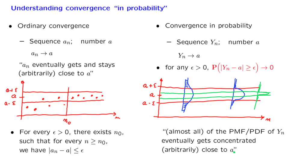
Convergence in probability
- Definition:
A sequence Y_n converges in probability to a number a if For any \epsilon > 0, \displaystyle \lim_{n\rightarrow\infty}\textbf{P}(|Y_n - a| \ge \epsilon) = 0 * Comparison between ordinary convergence and convergence in probability:
Convergence in probability examples
- convergence in probability doesn't imply convergence of the expectations.
- How to find what value it converges to? Make an educated conjecture about the limit \tau, write {\bf P}(|Y_n - \tau| \ge \epsilon), and derive the value of it to where you can observe from the expression that the probability \to 0, when n \to \infty.
Related topics
- Better bounds/approximations on tail probabilities
- Markov and Chebyshev inequalities
- Chernoff bound
- Central limit theorem
- Different types of convergence
- Convergence in probability
- Convergence "with probability 1"
- Strong law of large numbers
- Convergence of a sequence of distributions (CDFs) to a limiting CDF.
Lecture 19 The Central Limit Theorem (CLT)
- Considering the sum of random variable S_n = X_1 + X_2, + \cdots + X_n, (X_1, X_2, \cdots, X_n are i.i.d. with finite mean \mu and variance \sigma^2) Z_n = \frac{S_n - n\mu}{\sqrt{n}\sigma}, then we have the central limit Theorem,
Central Limit Theorem: For every z: \displaystyle \lim_{n \to \infty}\textbf{P}(Z_n \le z) = \textbf{P}(Z \le z)
What exactly does the CLT say? - Practice
- The practice of normal approximations:
We have linear expression between S_n and Z_n: S_n = \sqrt n \sigma Z_n + n\mu, since Z_n can be treated as if it were normal, S_n can be treated as if normal: N(n\mu, n\sigma^2)
- Can we use the CLT when n is "moderate"? i.e. n = 30?
- Usually, yes. When the distribution of X has common features with a normal distribution.
- symmetry and unimodality help
Central Limit Theory examples
- \textbf{P}(S_{\color{red}n} \le {\color{red}a}) \approx {\color{red}b} Given two parameters, find the third.
- Package weight X_i, i.i.d. exponential, \lambda = 1/2, \mu = \sigma = 2
- Load container with n = 100 packages, what's the probability that the overall weight is heavier than 210? \textbf{P}(S_n \ge 210) = ?
- Load container with n = 100 packages. Choose the "capacity" a so that \textbf{P}(S_n \ge a) \approx 0.05
- Fix the capacity at 210, how large can n be, so that \textbf{P}(S_n \ge 210) \approx 0.05
- Load container until wight exceeds 210, N is the number of packages loaded, find \textbf{P}(N > 100)
Airline booking
For any given flight, an airline tries to sell as many tickets as possible. Suppose that on average, of ticket holders fail to show up, all independent of one another. Knowing this, an airline will sell more tickets than there are seats available (i.e., overbook the flight) and hope that there is a sufficient number of ticket holders who do not show up, to compensate for its overbooking. Using the Central Limit Theorem, determine, the maximum number of tickets an airline can sell on a flight with 400 seats so that it can be approximately confident that all ticket holders who do show up will be able to board the plane. Use the de Moivre-Laplace -correction in your calculations. Hint: You may have to solve numerically a quadratic equation.
Solution: Each ticket can either be used or not used by the the passager. It can be modeled with the random variable: X \sim \operatorname{Bern} \left({p}\right), p=0.8, then the total passergers presented at airport is S_n = X_1 + X_2 + \cdots + X_n, which is a Binomial: S_n \sim \operatorname{B} \left({n, p}\right). For binomial random variable, \mu = np = 0.8n, \sigma^2 = np(1-p) = 0.16n. Our requirements is \textbf{P}(S_n \le 400) \approx 0.99. Normalize S_n in the probability and treat the normalized random variable Z_n as a normal distribution, refer to the normal table, and solve the number n.
Solve n to obtain n = 475
Normal approximation to the binomial
- Take X_i as independent Bernuolli random variables: X \sim \operatorname{Bern} \left({p}\right), 0 < p < 1, then S_n = X_1 + X_2 + \cdots + X_n is Binomial: X \sim \operatorname{B} \left({n, p}\right). Binomial random variable S_n have \mu = np, \sigma^2=np(1-p). According CLT, The normalized random variable \frac{S_n-np}{\sqrt{np(1-p)}} is a standard normal. In order to find the \textbf{P}(S_n \le 21) (given n = 36, p = 0.5), we use the equvilent of events to transform the probability \textbf{P}(S_n \le 21) into another probability about a normal random vairable \textbf{P}\Big(\frac{S_n - 18}{3} \le \frac{21-28}{3}\Big) = \textbf{P}(Z_n \le 1) = \Phi(1) = 0.8413.
- The 1/2 correction for integer random variables. To get a improved estimate of binomial from normal, we can take the middle point of two integers. Instead using \textbf{P}(S_n \le 21) or \textbf{P}(S_n \lt 22), we use \textbf{P}(S_n \lt 21.5) which is very accurate
- De Moivre-Laplace CLT to the binomial. To estimate \textbf{P}(S_n=19), we take \textbf{P}(18.5 \le S_n \le 19.5) and get an accurate estimate.
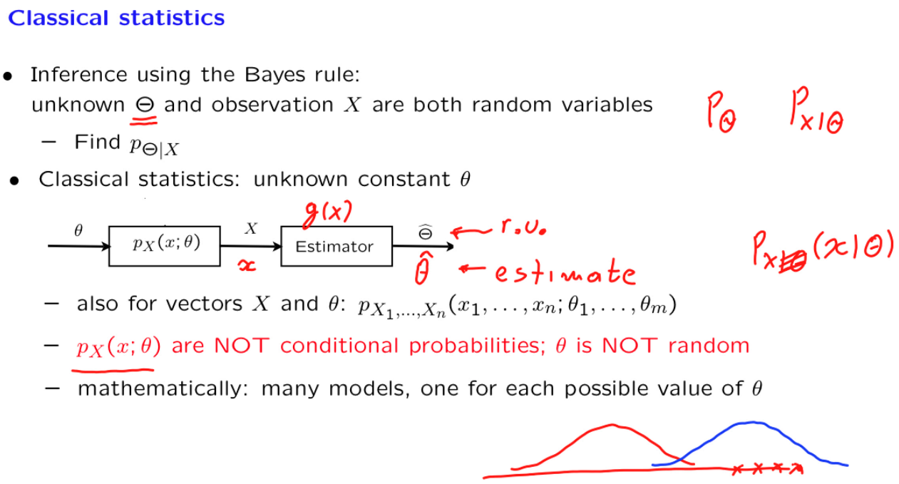
Lecture 20 Introduction to classical statistics
Overview of the classical statistical framework
| attributes | Bayesian | classical |
|---|---|---|
| unkonwn | \Theta is r.v. | \theta is a fixed value |
| known | p_\Theta prior distribution and samples X_i | only sample X_i |
| model | p_{X \mid \Theta}, where observation is generated | p_X(x; \theta),\theta is a real-valued parameter of the model, |
| method | use bayes rule to obtain p_{\Theta \mid X}, \big(p_X = {\int_{-\infty}^{+\infty}} p_\Theta \cdot p_{X \mid \Theta}d\theta\big), then determind the estimate | Design a estimator \hat\Theta, to keep estimate error \hat\Theta - \theta small |
| estimator | MAP, LMS | ML |
Confidence intervals interpretation
Every day, I try to estimate an unknown parameter using a fresh data set. I look at the data and then I use some formulas to calculate a 70% confidence interval, [\hat\Theta^-, \hat\Theta^+], based on the day's data.
Classical statsistic interpretation
If today I got the confidence interval [0.41, 0.47], that doesn't mean there is 70\% probability that the true value will be inside [0.41, 0.47]. What the confidence interval is that 70% of those confidence intervals you obtained in all those days will include the true value. The "confidence" (or probability) can be think of \frac{\text{All CIs that include the true value}}{\text{All CIs that include the true value + CIs that exclude the true value}}. You cannot speak about a particular interval, and once you do that, there is no randomness anymore, the true value is either inside the interval or not, there are no other probabilities so to speak.
Bayes' interpretation (Bayesian's Confidence Interval)
Alternatively, I decided to use a Bayesian approach, by viewing the unknown parameter, denoted by \Theta, as a continuous random variable and assuming a prior PDF for \Theta. I observe a specific value x, calculate the posterior f_{\Theta}{X}(\theta|x), and find out that
This time, I can say that there is a probability 70\% that the unknown parameter is inside the (Bayesian) confidence interval [0.41, 0.47].
Confidence intervals for the estimation of the mean
I asked you to estimate the mean of i.i.d variables X_1, X_2, \cdots, X_n with true mean \theta, and variance \sigma^2, and the estimate should achieve 95\% confidence interval. How you proceed with it?
- By Central Limit Theory, your estimate values \hat\Theta is an normal distribution. By standardizing it, you get the standard normal Z_n = \frac{\hat\Theta - \theta}{\sigma/\sqrt{n}}. 95\% confidence interverl means standard normal is between symetric 95\% intervals [-b, b]. By looking up the normal table, b = 1.69 corresponds to the probability 97.5\%, so \textbf{P}(-1.69 \le Z_n \le 1.69) = 95\% thus \textbf{P}\big(\frac{|\hat\Theta - \theta|}{\sigma/\sqrt{n}} \le 1.69\big) = 95\%, which can be rewrite as
This is the way to construct the confidence interval. If you have the \sigma and n, you have a concrete 95\% confidence interval to report.
However, the \sigma is usually unknown, what you can do is to use the estimated \hat\Theta to estimate the \sigma.