Concurrent Programming in Java¶

parallelStream() fork/join conditional variable

Week 1¶

1.1 Threads¶

Thread Example

// main thread T0
t1 = new Thread(s1); // s1 is the computation assign val x
t1.start();          // start thread t1 by main thread t0
s2;                  // execute computation task by t0
t1.join();           // wait the val x computation from t1 for use in s3
s3;                  // computation read val x

Deadlock

// If s1 have t2.join() and s1` have t1.join(), deadlock will happen
// main thread T0
t1 = new Thread(s1);   // s1 is the computation assign val x
t2 = new Thread(s1`);  // s1` is the computation assign val x
t1.start();            // start thread t1 by main thread t0
t2.start()             // start thread t2 by main thread t0
s2;                    // execute computation task by t0
t1.join();             // wait the val x computation from t1 for use in s3
s3;                    // computation read val x

1.1 Lecture Summary

In this lecture, we learned the concept of threads as lower-level building blocks for concurrent programs. A unique aspect of Java compared to prior mainstream programming languages is that Java included the notions of threads (as instances of the java.lang.Thread class in its language definition right from the start.

When an instance of Thread is created (via a new operation), it does not start executing right away; instead, it can only start executing when its start() method is invoked. The statement or computation to be executed by the thread is specified as a parameter to the constructor.

The Thread class also includes a wait operation in the form of a join() method. If thread t0 performs a t1.join() call, thread t0 will be forced to wait until thread t1 completes, after which point it can safely access any values computed by thread t1. Since there is no restriction on which thread can perform a join on which other thread, it is possible for a programmer to erroneously create a deadlock cycle with join operations. (A deadlock occurs when two threads wait for each other indefinitely, so that neither can make any progress.)

1.1 Optional Reading

1.2 Structured Locks¶

Synchronized

incr(A) {
  synchronized (A) {
    A.count = A.count + 1;
  } // release A
}

Unbounded Buffer

// x = {BUF, IN, OUT}
insert(item) {
  synchronized (x) {
    buf[in] = item;
    in++;
  }
}

remove() {
  synchronized (x) {
    item = buf[out];
    out++;
    return item;
  }
}

Bounded Buffer

// x = {BUF, IN, OUT} with size K
insert(item) {
  synchronized (x) {
    wait(); // wait if x is full
    buf[in] = item;
    in++;
    notify();
  }
}

remove() {
  synchronized (x) {
    wait(); // wait if x is empty
    item = buf[out];
    out++;
    notify();
    return item;
  }
}

1.2 Lecture Summary

In this lecture, we learned about structured locks, and how they can be implemented using synchronized statements and methods in Java. Structured locks can be used to enforce mutual exclusion and avoid data races, as illustrated by the incr() method in the A.count example, and the insert() and remove() methods in the the Buffer example. A major benefit of structured locks is that their acquire and release operations are implicit, since these operations are automatically performed by the Java runtime environment when entering and exiting the scope of a synchronized statement or method, even if an exception is thrown in the middle.

We also learned about wait() and notify() operations that can be used to block and resume threads that need to wait for specific conditions. For example, a producer thread performing an insert() operation on a bounded buffer can call wait() when the buffer is full, so that it is only unblocked when a consumer thread performing a remove() operation calls notify(). Likewise, a consumer thread performing a remove() operation on a bounded buffer can call wait() when the buffer is empty, so that it is only unblocked when a producer thread performing an insert() operation calls notify(). Structured locks are also referred to as intrinsic locks or monitors.

1.2 Optional Reading

Tutorial on Intrinsic Locks and Synchronization in Java
Tutorial on Guarded Blocks in Java
Wikipedia article on Monitors

1.3 Unstructured Locks¶

Hand-over-hand lock

// LinkedList: N1->N2->N3->N4
// Lock4Nodes: L1  L2  L3  L4
lock(L1);
lock(L2);
WORK with N1, N2
unlock(L1);
lock(L3);
WORK with N2, N3
unlock(L2);
lock(L4);
WORK with N3, N4
unlock(L3);

Hand-over-hand lock using try_lock

// LinkedList: N1->N2->N3->N4
// Lock4Nodes: L1  L2  L3  L4
try
  lock(L1);
if (success) {
  lock(L2);
  WORK with N1, N2
  unlock(L1);
  lock(L3);
  WORK with N2, N3
  unlock(L2);
  lock(L4);
  WORK with N3, N4
  unlock(L3);
}

R/W lock

// data: Array[]
// R/W lock: L
search (x) {
  read_lock(L)
  A[i] == x;  // read only
  unlock(L)
}

update(i, y) {
  write_lock(L)
  A[i] = y;   // write
  unlock(L)
}

1.3 Lecture Summary

In this lecture, we introduced unstructured locks (which can be obtained in Java by creating instances of ReentrantLock(), and used three examples to demonstrate their generality relative to structured locks. The first example showed how explicit lock() and unlock() operations on unstructured locks can be used to support a hand-over-hand locking pattern that implements a non-nested pairing of lock/unlock operations which cannot be achieved with synchronized statements/methods. The second example showed how the tryLock() operations in unstructured locks can enable a thread to check the availability of a lock, and thereby acquire it if it is available or do something else if it is not. The third example illustrated the value of read-write locks (which can be obtained in Java by creating instances of ReentrantReadWriteLock(), whereby multiple threads are permitted to acquire a lock L in "read mode", L.readLock().lock(), but only one thread is permitted to acquire the lock in “write mode”, L.writeLock().lock().

However, it is also important to remember that the generality and power of unstructured locks is accompanied by an extra responsibility on the part of the programmer, e.g., ensuring that calls to unlock() are not forgotten, even in the presence of exceptions.

1.3 Optional Reading

1.4 Liveness¶

Deadlock

// T1
synchronized (A) {
  synchronized (B) {
  }
}
// T2
synchronized (B) {
  synchronized (A) {
  }
}

Livelock

// T1
do {
  synchronized (B) {
    x.incr();
    r = x.get();
  }
} while (R < 2)
// T2
do {
  synchronized (B) {
    x.decr();
    r = x.get();
  }
} while (R > -2)

Starvation

// T1
do {
  int1 = s1.readline();
  print int1;
} while (...)
// ...
// T100
do {
  int100 = s100.readline();
  print int100;
} while (...)

1.4 Lecture Summary

In this lecture, we studied three ways in which a parallel program may enter a state in which it stops making forward progress. For sequential programs, an "infinite loop" is a common way for a program to stop making forward progress, but there are other ways to obtain an absence of progress in a parallel program. The first is deadlock, in which all threads are blocked indefinitely, thereby preventing any forward progress. The second is livelock, in which all threads repeatedly perform an interaction that prevents forward progress, e.g., an infinite “loop” of repeating lock acquire/release patterns. The third is starvation, in which at least one thread is prevented from making any forward progress.

The term "liveness" refers to a progress guarantee. The three progress guarantees that correspond to the absence of the conditions listed above are deadlock freedom, livelock freedom, and starvation freedom.

1.4 Optional Reading

Deadlock example with synchronized methods in Java
Starvation and Livelock examples in Java
Wikipedia article on Deadlock and Livelock

1.5 Dining Philosophers¶

think
pick up chopsticks (left, right)
eat
put down chopsticks

Structured locks

// if all pick up the left first, deadlock
while (...) {
  Think;
  sychronized (Left) {
    sychronized (Right) {
      Eat;
    }
  }
}

unstructured locks

// if all pick up the left first, livelock, but no deadlock
while (...) {
  Think;
  s1 = tryLock(Left);
  if (!s1) continue;
  s2 = tryLock(Right);
  if (!s2) {
    unlock(Left);
    continue;
  }
  Eat;
}

Modified version

// have one of the philosophers pick right first and then left.
// However, this can also cause the starvation problem. To solve
// the problem completely, we need to use another synchronization
// premitive called semaphore.

1.5 Lecture Summary

In this lecture, we studied a classical concurrent programming example that is referred to as the Dining Philosophers Problem. In this problem, there are five threads, each of which models a "philosopher" that repeatedly performs a sequence of actions which include think, pick up chopsticks, eat, and put down chopsticks.

First, we examined a solution to this problem using structured locks, and demonstrated how this solution could lead to a deadlock scenario (but not livelock). Second, we examined a solution using unstructured locks with tryLock() and unlock() operations that never block, and demonstrated how this solution could lead to a livelock scenario (but not deadlock). Finally, we observed how a simple modification to the first solution with structured locks, in which one philosopher picks up their right chopstick and their left, while the others pick up their left chopstick first and then their right, can guarantee an absence of deadlock.

1.5 Optional Reading

Wikipedia article on the Dining Philosophers Problem

1.6 Mini Project¶

The mini project used Java ReentrantLock and ReentrantReadWriteLock to ensure the list operations are free of bugs if run by multiple threads. One practical tip is that when using the basic lock primitive the lock statement can be put in the try and unlock in the finally statement, respectively.

Week 2¶

2.1 Critical Sections (Isloated Construct)¶

Balance Transfer

// My balance:       5000
// Family balance:   1000
// Daughter balance: 0
T1 {
  myBal = myBal - 100;         // R1
  familyBal = familyBal + 100; // W1
}

T2 {
  familyBal = familyBal - 100; // R2
  DauBal = DarBal + 100;       // W2
}

Use isolated

// My balance:       5000
// Family balance:   1000
// Daughter balance: 0
T1 {
  isolated {
    myBal = myBal - 100;         // R1
    familyBal = familyBal + 100; // W1
  }
}

T2 {
  isolated {
    familyBal = familyBal - 100; // R2
    DauBal = DarBal + 100;       // W2
  }
}

2.1 Lecture Summary

In this lecture, we learned how critical sections and the isolated construct can help concurrent threads manage their accesses to shared resources, at a higher level than just using locks. When programming with threads, it is well known that the following situation is defined to be a data race error — when two accesses on the same shared location can potentially execute in parallel, with least one access being a write. However, there are many cases in practice when two tasks may legitimately need to perform concurrent accesses to shared locations, as in the bank transfer example.

With critical sections, two blocks of code that are marked as isolated, say A and B, are guaranteed to be executed in mutual exclusion with A executing before B or vice versa. With the use of isolated constructs, it is impossible for the bank transfer example to end up in an inconsistent state because all the reads and writes for one isolated section must complete before the start of another isolated construct. Thus, the parallel program will see the effect of one isolated section completed before another isolated section can start.

2.1 Optional Reading

Wikipedia article on Critical Sections
Wikipedia article on Atomicity

2.2 Object Based Isolation (Monitors)¶

DoubleLinkedList Example

// A <-> B <-> C <-> D <-> E
delete(cur) {
  cur.prev.next = cur.next;
  cur.next.prev = cur.prev;
}
// T1: Delete(B)
// T2: Delete(C)
// T3: Delete(E)

DoubleLinkedList using isolated

// A <-> B <-> C <-> D <-> E
delete(cur) {
  isolated (cur, cur.prev, cur.next) {
    cur.prev.next = cur.next;
    cur.next.prev = cur.prev;
  }
}
// T1: Delete(B) touch (A, B, C)
// T2: Delete(C) touch (B, C, D)
// T3: Delete(E) touch (D, E, F)
// T1 and T3 can be done in the same time.

Monitor intuition

// P1, process 1
// P2, process 2
Isolated(M1)
M1 {
  P1: Isolated(M1);
  P2: Isolated(M1);
}
M2 {
  P1: Isolated(M2);
  P2: Isolated(M2);
}
Isolated(M2)

2.2 Lecture Summary

In this lecture, we studied object-based isolation, which generalizes the isolated construct and relates to the classical concept of monitors. The fundamental idea behind object-based isolation is that an isolated construct can be extended with a set of objects that indicate the scope of isolation, by using the following rules: if two isolated constructs have an empty intersection in their object sets they can execute in parallel, otherwise they must execute in mutual exclusion. We observed that implementing this capability can be very challenging with locks because a correct implementation must enforce the correct levels of mutual exclusion without entering into deadlock or livelock states. The linked-list example showed how the object set for a delete() method can be defined as consisting of three objects — the current, previous, and next objects in the list, and that this object set is sufficient to safely enable parallelism across multiple calls to delete(). The Java code sketch to achieve this object-based isolation using the PCDP library is as follows:

isolated(cur, cur.prev, cur.next, () -> {
    . . . // Body of object-based isolated construct
});

The relationship between object-based isolation and monitors is that all methods in a monitor object, M1, are executed as object-based isolated constructs with a singleton object set, M1. Similarly, all methods in a monitor object, M2, are executed as object-based isolated constructs with a singleton object set, M2 which has an empty intersection with M1.

2.2 Optional Reading

Wikipedia article on Monitors

2.3 Concurrent Spanning Tree Algorithm¶

Spanning Tree Algorithm

Compute(v) {
  for each neighbor c of v
    s <- MakeParent(v, c)
    if (s)
      Compute(c);
}

MakeParent(v, c) {
  if (c.parent == Null) {
    c.parent = v;
    success = true;
  } else {
    success = false;
    return success;
  }
}

Isolation Construct

Compute(v) {
  for each neighbor c of v
    s <- MakeParent(v, c)
    if (s)
      Compute(c);
}

MakeParent(v, c) {
  isolated(c) {
    if (c.parent == Null) { // compare-and-set premitive
      c.parent = v;
      success = true;
    } else {
      success = false;
      return success;
    }
  }
}

2.3 Lecture Summary

In this lecture, we learned how to use object-based isolation to create a parallel algorithm to compute spanning trees for an undirected graph. Recall that a spanning tree specifies a subset of edges in the graph that form a tree (no cycles), and connect all vertices in the graph. A standard recursive method for creating a spanning tree is to perform a depth-first traversal of the graph (the Compute(v) function in our example), making the current vertex a parent of all its neighbors that don’t already have a parent assigned in the tree (the MakeParent(v, c) function in the example).

The approach described in this lecture to parallelize the spanning tree computation executes recursive Compute(c) method calls in parallel for all neighbors, c, of the current vertex, v. Object-based isolation helps avoid a data race in the MakeParent(v,c) method, when two parallel threads might attempt to call MakeParent(v1, c) and MakeParent(v2, c) on the same vertex c at the same time. In this example, the role of object-based isolation is to ensure that all calls to MakeParent(v,c) with the same c value must execute the object-based isolated statement in mutual exclusion, whereas calls with different values of c can proceed in parallel.

2.3 Optional Reading

Wikipedia article on Spanning Trees

2.4 Atomic Variables¶

Atomic Variables (Integer)

// X[0, ... N-1]
do {
  j = curr;       // curr.getAndAdd(1); atomic integer!!!.
  cur = cur + 1;
  if (j >= N) break;
  process(X[j])
} while (true)

Atomic Reference (compareAndSet)

compareAndSet(expected, new) {
  isolated (this) {
    if (this.val == expected) {
      this.val = new;
      return true;
    } else {
      return false;
    }
  }
}

2.4 Lecture Summary

In this lecture, we studied Atomic Variables, an important special case of object-based isolation which can be very efficiently implemented on modern computer systems. In the example given in the lecture, we have multiple threads processing an array, each using object-based isolation to safely increment a shared object, cur, to compute an index j which can then be used by the thread to access a thread-specific element of the array.

However, instead of using object-based isolation, we can declare the index cur to be an Atomic Integer variable and use an atomic operation called getAndAdd() to atomically read the current value of cur and increment its value by 1. Thus, j = cur.getAndAdd(1) has the same semantics as isolated (cur) { j = cur; cur = cur+1;} but is implemented much more efficiently using hardware support on today’s machines.

Another example that we studied in the lecture concerns Atomic Reference variables, which are reference variables that can be atomically read and modified using methods such as compareAndSet(). If we have an atomic reference ref, then the call to ref.compareAndSet(expected, new) will compare the value of ref to expected, and if they are the same, set the value of ref to new and return true. This all occurs in one atomic operation that cannot be interrupted by any other methods invoked on the ref object. If ref and expected have different values, compareAndSet() will not modify anything and will simply return false.

2.4 Optional Reading

Tutorial on Atomic Integers in Java
Article in Java theory and practice series on Going atomic
Wikipedia article on Atomic Wrapper Classes in Java

2.5 Read, Write Isolation¶

Read/Write Isolation

// T1: C.Get(k1), C.Get(k3), C.Get(k5)
// T2: C.Get(k1), C.Get(k3), C.Get(k5)
// T3: C.Put(k1)
isolated (read(C)) {
  V = C.get(k1);
}

isolated (write(C)) {
  C.put(k2, v2);
}

Read/Write Isolation in LinkedList example

delete (cur) {
  isolated (write(cur.next, cur.prev), read(cur)) {
    cur.prev.next = cur.next;
    cur.next.prev = cur.prev;
  }
}

2.5 Lecture Summary

In this lecture we discussed Read-Write Isolation, which is a refinement of object-based isolation, and is a higher-level abstraction of the read-write locks studied earlier as part of Unstructured Locks. The main idea behind read-write isolation is to separate read accesses to shared objects from write accesses. This approach enables two threads that only read shared objects to freely execute in parallel since they are not modifying any shared objects. The need for mutual exclusion only arises when one or more threads attempt to enter an isolated section with write access to a shared object.

This approach exposes more concurrency than object-based isolation since it allows read accesses to be executed in parallel. In the doubly-linked list example from our lecture, when deleting an object cur from the list by calling delete(cur), we can replace object-based isolation on cur with read-only isolation, since deleting an object does not modify the object being deleted; only the previous and next objects in the list need to be modified.

2.5 Optional Reading

Wikipedia article on Readers-writer lock

2.6 Mini project¶

Week 3¶

Akka

3.1 Actors¶

getAndAdd(){
  j = cur;
  cur = cur + delta;
  return j;
}

// method doesn't doing correct isolation
foo () {
  cur = ...  
}

Actor (reactive)

Mailbox
Method
Local State

3.1 Lecture Summary

In this lecture, we introduced the Actor Model as an even higher level of concurrency control than locks or isolated sections. One limitation of locks, and even isolated sections, is that, while many threads might correctly control the access to a shared object (e.g., by using object-based isolation) it only takes one thread that accesses the object directly to create subtle and hard-to-discover concurrency errors. The Actor model avoids this problem by forcing all accesses to an object to be isolated by default. The object is part of the local state of an actor, and cannot be accessed directly by any other actor.

An Actor consists of a Mailbox, a set of Methods, and Local State. The Actor model is reactive, in that actors can only execute methods in response to messages; these methods can read/write local state and/or send messages to other actors. Thus, the only way to modify an object in a pure actor model is to send messages to the actor that owns that object as part of its local state. In general, messages sent to actors from different actors can be arbitrarily reordered in the system. However, in many actor models, messages sent between the same pair of actors preserve the order in which they are sent.

3.1 Optional Reading

Wikipedia article on the Actor Model
Documentation on the Akka Actor Library (though Akka is not used in this course, it is a useful library to be aware of if you are interested in using the actor model with Java and Scala applications)

3.2 Actor Examples¶

// print actor
process (s) { // like a callback
  if (s == "Exit")
    exit();
  else
    print s;
}

actor-example

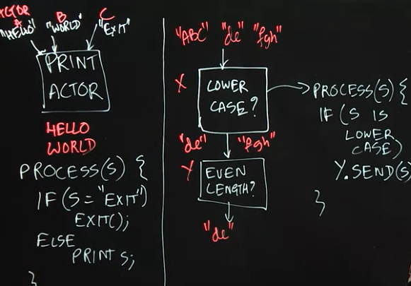
3.2 Lecture Summary

In this lecture, we further studied the Actor Model through two simple examples of using actors to implement well-known concurrent programming patterns. The PrintActor in our first example processes simple String messages by printing them. If an EXIT message is sent, then the PrintActor completes its current computation and exits. As a reminder, we assume that messages sent between the same pair of actors preserve the order in which they are sent.

In the second example, we created an actor pipeline, in which one actor checks the incoming messages and only forwards the ones that are in lower case. The second actor processes the lowercase messages and only forwards the ones that are of even length. This example illustrates the power of the actor model, as this concurrent system would be much more difficult to implement using threads, for example, since much care would have to be taken on how to implement a shared mailbox for correct and efficient processing by parallel threads.

3.2 Optional Reading

Wikipedia article on Pipeline Parallelism.

3.3 Sieve of Eratosthenes Algorithm¶

actor-example

3.3 Lecture Summary

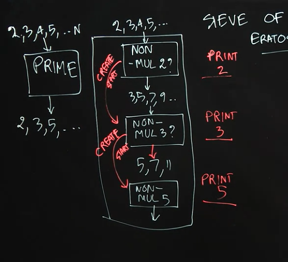
In this lecture, we studied how to use actors to implement a pipelined variant of the Sieve of Eratosthenes algorithm for generating prime numbers. This example illustrates the power of the Actor Model, including dynamic creation of new actors during a computation.

To implement the Sieve of Eratosthenes, we first create an actor, Non-Mul-2, that receives (positive) natural numbers as input (up to some limit), and then filters out the numbers that are multiples of 2. After receiving a number that is not a multiple of 2 (in our case, the first would be 3), the Non-Mul-2 actor creates the next actor in the pipeline, Non-Mul-3, with the goal of discarding all the numbers that are multiples of 3. The Non-Mul-2 actor then forwards all non-multiples of 2 to the Non-Mul-3 actor. Similarly, this new actor will create the next actor in the pipeline, Non-Mul-5, with the goal of discarding all the numbers that are multiples of 5. The power of the Actor Model is reflected in the dynamic nature of this problem, where pieces of the computation (new actors) are created dynamically as needed.

A Java code sketch for the process() method for an actor responsible for filtering out multiples of the actor's "local prime" in the Sieve of Eratosthenes is as follows:

public void process(final Object msg) {
  int candidate = (Integer) msg;
  // Check if the candidate is a non-multiple of the "local prime".
  // For example, localPrime = 2 in the Non-Mul-2 actor
  boolean nonMul = ((candidate % localPrime) != 0);
  // nothing needs to be done if nonMul = false
  if (nonMul) {
    if (nextActor == null) {
      . . . // create & start new actor with candidate as its local prime
    }
    else nextActor.send(msg); // forward message to next actor
  }
} // process

3.3 Optional Reading

Wikipedia article on the Sieve of Eratosthenes problem

3.4 Producer-Consumer Problem¶

// consumer thread
while (buffer.empty()) { }
// process item removed from buffer

producer-consumer-problem

3.4 Lecture Summary

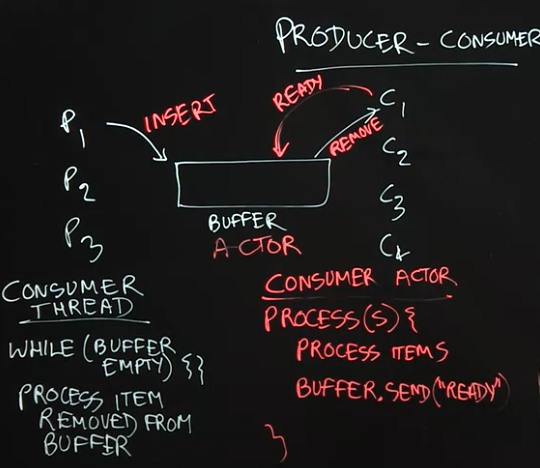
In this lecture, we studied the producer-consumer pattern in concurrent programming which is used to solve the following classical problem: how can we safely coordinate accesses by multiple producer tasks, $P_1$ , $P_2$ , $P_3$ ... and multiple consumer tasks, $C_1$ , $C_2$ , $C_3$ , ... to a shared buffer of unbounded size without giving up any concurrency? Part of the reason that this problem can be challenging is that we cannot assume any a priori knowledge about the rate at which different tasks produce and consume items in the buffer. While it is possible to solve this problem by using locks with wait-notify operations or by using object-based isolation, both approaches will require low-level concurrent programming techniques to ensure correctness and maximum performance. Instead, a more elegant solution can be achieved by using actors as follows.

The key idea behind any actor-based solution is to think of all objects involved in the concurrent program as actors, which in this case implies that producer tasks, consumer tasks, and the shared buffer should all be implemented as actors. The next step is to establish the communication protocols among the actors. A producer actor can simply send a message to the buffer actor whenever it has an item to produce. The protocol for consumer actors is a bit more complicated. Our solution requires a consumer actor to send a message to the buffer actor whenever it is ready to process an item. Thus, whenever the buffer actor receives a message from a producer, it knows which consumers are ready to process items and can forward the produced item to any one of them. Thus, with the actor model, all concurrent interactions involving the buffer can be encoded in messages, instead of using locks or isolated statements.

3.5 Bounded Buffer Problem¶

bounded-buffer-problem

3.5 Lecture Summary

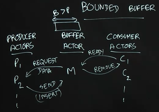
A major simplification made in the previous lecture was to assume that the shared buffer used by producer and consumer tasks can be unbounded in size. However, in practice, it is also important to consider a more realistic version of the the producer-consumer problem in which the buffer has a bounded size. In fact, the classical producer-consumer problem statement usually assumes a bounded buffer by default. In this lecture, we studied how the actor-based solution to the unbounded buffer case can be extended to support a bounded buffer.

The main new challenge with bounding the size of the shared buffer is to ensure that producer tasks are not permitted to send items to the buffer when the buffer is full. Thus, the buffer actor needs to play a master role in the protocol by informing producer actors when they are permitted to send data. This is akin to the role played by the buffer/master actor with respect to consumer actors, even in the unbounded buffer case (in which the consumer actor informed the buffer actor when it is ready to consume an item). Now, the producer actor will only send data when requested to do so by the buffer actor. Though, this actor-based solution appears to be quite simple, it actually solves a classical problem that has been studied in advanced operating system classes for decades.

3.5 Optional Reading

Wikipedia article on the Producer-Consumer problem

Week 4¶

4.1 Optimistic concurrency¶

class Integer {
  get();
  set();
  getAndAdd(delta) {
    curr = this.get();
    next = cur + delta;
    this.set(next);  // RACE CONDITION
    return cur;
  }
}

class AutomicInteger {
  get();
  set();
  compareAndSet();
  getAndAdd(delta) {
    while(true) {
      curr = this.get();
      next = cur + delta;
      if (this.compareAndSet(curr, next)) {
        return cur;
      }
    }
  }
}

4.1 Lecture Summary

In this lecture, we studied the optimistic concurrency pattern, which can be used to improve the performance of concurrent data structures. In practice, this pattern is most often used by experts who implement components of concurrent libraries, such as AtomicInteger and ConcurrentHashMap, but it is useful for all programmers to understand the underpinnings of this approach. As an example, we considered how the getAndAdd() method is typically implemented for a shared AtomicInteger object. The basic idea is to allow multiple threads to read the existing value of the shared object (curVal) without any synchronization, and also to compute its new value after the addition (newVal) without synchronization. These computations are performed optimistically under the assumption that no interference will occur with other threads during the period between reading curVal and computing newVal. However, it is necessary for each thread to confirm this assumption by using the compareAndSet() method as follows. (compareAndSet() is used as an important building block for optimistic concurrency because it is implemented very efficiently on many hardware platforms.)

The method call A.compareAndSet(curVal, newVal) invoked on AtomicInteger A checks that the value in A still equals curVal, and, if so, updates A’s value to newVal before returning true; otherwise, the method simply returns false without updating A. Further, the compareAndSet() method is guaranteed to be performed atomically, as if it was in an object-based isolated statement with respect to object A. Thus, if two threads, $T_1$ and $T_2$ call compareAndSet() with the same curVal that matches A’s current value, only one of them will succeed in updating A with their newVal. Furthermore, each thread will invoke an operation like compareAndSet() repeatedly in a loop until the operation succeeds. This approach is guaranteed to never result in a deadlock since there are no blocking operations. Also, since each call compareAndSet() is guaranteed to eventually succeed, there cannot be a livelock either. In general, so long as the contention on a single shared object like A is not high, the number of calls to compareAndSet() that return false will be very small, and the optimistic concurrency approach can perform much better in practice (but at the cost of more complex code logic) than using locks, isolation, or actors.

4.1 Optional Reading

Wikipedia article on Optimistic concurrency control
Documentation on Java’s AtomicInteger class

4.2 Concurrent Queue¶

Queue {
  enQ(x) {
    tail.next = x;
    tail = x;
  }

  deQ() {
    if (Q.empty) {// exception }
    r = head;
    head = head.next;
    return r;
  }
}

Queue {
  enQ(x) {
    while (true) {
      if (!tail.next.compareAndSet(null, x)) {
        continue;
      }
    }
  }

  deQ() {
    if (Q.empty) {// exception }
    r = head;
    head = head.next;
    return r;
  }
}

4.2 Lecture Summary

In this lecture, we studied concurrent queues, an extension of the popular queue data structure to support concurrent accesses. The most common operations on a queue are enq(x), which enqueues object x at the end (tail) of the queue, and deq() which removes and returns the item at the start (head) of the queue. A correct implementation of a concurrent queue must ensure that calls to enq() and deq() maintain the correct semantics, even if the calls are invoked concurrently from different threads. While it is always possible to use locks, isolation, or actors to obtain correct but less efficient implementations of a concurrent queue, this lecture illustrated how an expert might implement a more efficient concurrent queue using the optimistic concurrency pattern.

A common approach for such an implementation is to replace an object reference like tail by an AtomicReference. Since the compareAndSet() method can also be invoked on AtomicReference objects, we can use it to support (for example) concurrent calls to enq() by identifying which calls to compareAndSet() succeeded, and repeating the calls that failed. This provides the basic recipe for more efficient implementations of enq() and deq(), as are typically developed by concurrency experts. A popular implementation of concurrent queues available in Java is java.util.concurrent.ConcurrentLinkedQueue.

4.2 Optional Reading

4.3 Linearizability¶

4.3 Lecture Summary

In this lecture, we studied an important correctness property of concurrent objects that is called Linearizability. A concurrent object is a data structure that is designed to support operations in parallel by multiple threads. The key question answered by linearizability is what return values are permissible when multiple threads perform these operations in parallel, taking into account what we know about the expected return values from those operations when they are performed sequentially. As an example, we considered two threads, $T_1$ and $T_2$ , performing enq(x) and enq(y) operations in parallel on a shared concurrent queue data structure, and considered what values can be returned by a deq() operation performed by $T_2$ after the call to enq(y). From the viewpoint of linearizability, it is possible for the deq() operation to return item x or item y.

One way to look at the definition of linearizability is as though you are a lawyer attempting to "defend" a friend who implemented a concurrent data structure, and that all you need to do to prove that your friend is "not guilty" (did not write a buggy implementation) is to show one scenario in which all the operations return values that would be consistent with a sequential execution by identifying logical moments of time at which the operations can be claimed to have taken effect. Thus, if deq() returned item x or item y you can claim that either scenario is plausible because we can reasonably assume that enq(x) took effect before enq(y), or vice versa. However, there is absolutely no plausible scenario in which the call to deq() can correctly return a code/exception to indicate that the queue is empty since at least enq(y) must have taken effect before the call to deq(). Thus, a goal for any implementation of a concurrent data structure is to ensure that all its executions are linearizable by using whatever combination of constructs (e.g., locks, isolated, actors, optimistic concurrency) is deemed appropriate to ensure correctness while giving the maximum performance.

4.3 Optional Reading

Wikipedia article on the Linearizability

4.4 ConcurrentHashMap¶

java.util.concurrent.ConcurrentHashMap.get(key);
java.util.concurrent.ConcurrentHashMap.put(key, value);
java.util.concurrent.ConcurrentHashMap.putIfAbsent(key, value);
java.util.concurrent.ConcurrentHashMap.clear(key, value);
java.util.concurrent.ConcurrentHashMap.putAll(key, value);

java.util.concurrent.ConcurrentLinkedQueue
java.util.concurrent.ConcurrentSkipListSet

4.4 Lecture Summary

In this lecture, we studied the ConcurrentHashMap data structure, which is available as part of the java.util.concurrent standard library in Java. A ConcurrentHashMap instance, chm, implements the Map interface, including the get(key) and put(key, value) operations. It also implements additional operations specified in the ConcurrentMap interface (which in turn extends the Map interface); one such operation is putIfAbsent(key, value). The motivation for using putIfAbsent() is to ensure that only one instance of key is inserted in chm, even if multiple threads attempt to insert the same key in parallel. Thus, the semantics of calls to get(), put(), and putIfAbsent() can all be specified by the theory of linearizability studied earlier. However, it is worth noting that there are also some aggregate operations, such as clear() and putAll(), that cannot safely be performed in parallel with put(), get() and putIfAbsent().

Motivated by the large number of concurrent data structures available in the java.util.concurrent library, this lecture advocates that, when possible, you use libraries such as ConcurrentHashMap rather than try to implement your own version.

4.4 Optional Reading

Documentation on Java’s ConcurrentHashMap class
Wikipedia article on Java’s ConcurrentMap interface

4.5 Concurrent Minimum Spanning Tree Algorithm¶

// Boruvka MST
// L is the vertices set (ConcurrentLinkedQueue)
while (size() > 1) {
  n1 = remove(L);
  if (!tryLock(n1)) { continue; }
  e = getMinEdge(M);
  n2 = getNeighbor(n1, e);
  if (!tryLock(n2)) {
    // fixup
    continue;
  }
  n3 = merge(n1, n2);
  remove(n2);
  insert(n3);
}

4.5 Lecture Summary

In this lecture, we discussed how to apply concepts learned in this course to design a concurrent algorithm that solves the problem of finding a minimum-cost spanning tree (MST) for an undirected graph. It is well known that undirected graphs can be used to represent all kinds of networks, including roadways, train routes, and air routes. A spanning tree is a data structure that contains a subset of edges from the graph which connect all nodes in the graph without including a cycle. The cost of a spanning tree is computed as the sum of the weights of all edges in the tree.

The concurrent algorithm studied in this lecture builds on a well-known sequential algorithm that iteratively performs edge contraction operations, such that given a node N1 in the graph, GetMinEdge(N1) returns an edge adjacent to N1 with minimum cost for inclusion in the MST. If the minimum-cost edge is (N1,N2), the algorithm will attempt to combine nodes N1 and N2 in the graph and replace the pair by a single node, N3. To perform edge contractions in parallel, we have to look out for the case when two threads may collide on the same vertex. For example, even if two threads started with vertices A and D, they may both end up with C as the neighbor with the minimum cost edge. We must avoid a situation in which the algorithm tries to combine both A and C and D and C. One possible approach is to use unstructured locks with calls to tryLock() to perform the combining safely, but without creating the possibility of deadlock or livelock situations. A key challenge with calling tryLock() is that some fix-up is required if the call returns false. Finally, it also helps to use a concurrent queue data structure to keep track of nodes that are available for processing.

4.5 Optional Reading

Wikipedia article on Borvka’s algorithm for finding a minimum cost spanning tree of an undirected graph