CS224N NLP with Deep Learning¶

Part 1 Word Embeddings Based on Distributional Semantic¶

Date: April 20th 2019

If you have no experience in the Natrual Language Processing (NLP) field and asked to name a few practical NLP applications, what would you list? Google Translation or Amazon Echo voice assistant may first come into your mind. How did those products understand a sentence or human conversation? Engineers built computational models that understand our language as our brain does. To build such a computational model, the following components are necessary.

1. A large corpus of text (input training data)
2. A method to represent each word from the corpus (feature representation)
3. A starting model that barely understands English at the beginning but can be improved by "reading" more words from the corpus (parametric function).
4. An algorithm for the model to correct itself if it makes a mistake in understanding (learning algorithm/optimization method)
5. A measurement that can qualify the mistake the model made (loss function)

Introduction¶

Starting with this post, I will write materials from my understanding of the Stanford CS224N. The plan is to journal down all the learning notes I learned about the above 5 components. The goal is to provide a systematic understand of the gist of the components for real applications.

• Part 1 is about language models and word embeddings.
• Part 2 discusses neural networks and backpropagation algorithm.
• Part 3 revisits the language model and introduces recurrent neural networks.
• Part 4 studies advanced RNN, Long short-term memory (LSTM), and gated recurrent networks (GRN).

Word representations¶

How do we represent word with meaning on a computer? Before 2013, wordNet and one-hot vector are most popular in word meaning representations. WordNet is a manually compiled thesaurus containing lists of synonym sets and hypernyms. Like most of the manual stuff, it is subjective, unscalable, inaccurate in computing word similarity, and impossible to maintain and keep up-to-data. One-hot vectors represent word meaning using discrete symbolic $1$s in a long stream of $0$ of vector elements. It suffers from sparsity issues and many other drawbacks. We will not spend time on that outdated method. Instead, we will focus on the embedding method using the idea of word vector.

The core idea of this embedding method is based on the remarkable insight on word meaning called distributional semantics. It conjectures that a word’s meaning is given by the words that frequently appear close-by. It is proposed by J. R. Firth. Here is the famous quote:

In this method, we will build a dense vector for each word, chosen so that it is similar to vectors of words that appear in similar contexts. word vector representation also called distributed representation, or word embeddings. A work vector might look likes this,

word2vec¶

Word2vec (Mikolov et al. 2013) is a framework for learning word vectors. Word2vec go through windows of words and calculate the probability of the context word given the center word (or vice versa) using the similarity of the word vectors. It keeps adjusting the word vectors to maximize this probability. Vividly, these two pictures show the general idea of how word2vec works.

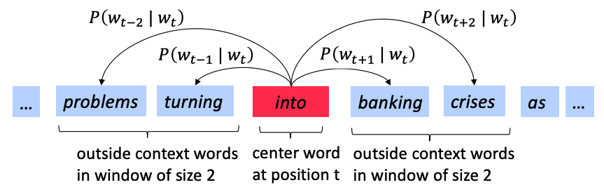
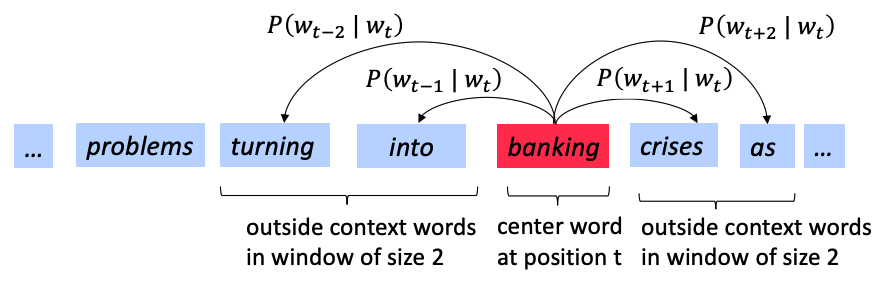
Formally, for a single prediction, the probability is $P(o|c)$, interpreted as the probability of the outer word $o$ given the center word $c$. For the large corpus including $T$ words and each position $t = 1, 2, \cdots, T$, we predict context words within a window of fixed size $m$, given center word $w_t$. The model likelihood can be written as the following

The objective function $J(\theta)$ is the average negative log likelihood:

We've defined the cost function by now. In order to minimize the loss, we need to know how $p(w_{t+j}|w_t; \theta)$ can be calculated. One function we can use to calculate the probability value is the $\mathrm{softmax}$ function.

Particularly we will write the probability as the following format.

There are several points need to be emphasized.

• Two vectors will be obtained for each individual word, one as center word $v_w$, and the other context word $u_w$. $d$ is the dimension of the word vector. $V$ is the vocabulary size.

• The dot product in the exponet compares similarity of $o$ and $c$. Larger dot product indicates larger probability.
• The denorminator sum over entire vocabulary to give normalized probability distribution.
• The $\mathrm{softmax}$ function maps aribitrary values $x_i$ to a probability distribution $p_i$. “$\mathrm{max}$” because it amplifies the probability of the largest $x_i$, “$\mathrm{soft}$” because it still assigns some probabilities to smaller $x_i$. It is very commonly used in deep learning.

Gradient descent to optimize log likelihood loss function¶

This section I will purely focus on how to derive the gradient of the log likelihood loss function with respect to center word using the chain rule. Once we have the computed gradients, we are ready to implement it in matrix form and train the word vectors. This model is called skip-gram.

• loss function in $p(w_{t+j}|w_t)$

• $p(w_{t+j}|w_t)$ in softmax form

We would like to find the following derivatives:

Let's now start working with the first one, the derivative wrt. $v_c$.

The result is remarkable. It have great intuition in it. The gradient represent the slop in the multidimentional space that we should walk along to reach the optima. The result gradient we got tell us that the slop equals to the difference of current context vector $\boldsymbol{u}_o$ and the expected context vector (the weighted average over all context vectors). It has nothing todo with the center word $c$.

To compute the gradient of $J(\theta)$ with respect to the center word $c$, you have to sum up all the gradients obtained from word windows when $c$ is the center word. The gradient with respect to the context word will be very similar, the chain rule is also handy in that case.

Once all the gradient with respect to center words and context words are calculated. We can use gradient descent to update the model parameters, which in this case is all the word vectors. Because we have two vectors for each word, when update the parameters we will use the average of the two vectors to update.

Gradient descent to optimize cross entropy loss function¶

Alternatively, we could also use cross entropy loss function. CS224N 2017 assignment 1 requires to derive the gradient of cross entropy loss function. This section, we will go step by step to derive the gradient when using cross entropy loss function and $\mathrm{softmax}$ activation function in the out put layer. the cross entropy function is defined as follows

Notice the $\boldsymbol{y}$ is the one-hot label vector, and $\boldsymbol{\hat y}$ is the predicted probability for all classes. The index $i$ is the index of the one-hot element in individual label vectors. Therefore the definition of cross entropy loss function is defined as followinng if we use $\mathrm{softmax}$ to predict $\hat y_i$,

The gradient of $\frac{\partial}{\partial \theta}J_{\mathrm{CE}}(\theta)$ can be derived using chain rule. Because we will use the gradient of the $\mathrm{softmax}$ for the derivation, Let's derive $\mathrm{softmax}$ gradient first.

Here we should use two tricks to derive this gradient.

1. Quotient rule
2. separate into 2 cases: when $i = j$ and $i \ne j$.

If $i = j$, we have

if $i \ne j$, we have

Now let calculate the gradient of the cross-entropy loss function. Notice the gradient is concerning the $i$th parameter. This is because we can use the gradient of the $\mathrm{softmax}$ (the $\frac{\partial \hat y_k}{\partial \theta_i}$ term) conveniently.

Write in vector form, we will have

With this gradient, we can update the model parameters, namely the word vectors. In the next post, I will discuss neural networks, which have more layers than the word2vec. In neural networks, there are more parameters need to be trained and the gradients with respect all the parameters need to be derived.

Skip-gram model¶

Skip-gram model uses the center word to predict the surrounding.

We have derived the gradient for the skip-gram model using log-likelihood loss function and $\mathrm{softmax}$. This section will derive the gradient for cross-entropy loss function. The probability output function will keep using the $\mathrm{softmax}$.

Cross entropy loss function¶

Since we have derived above that $\frac{\partial J_{\mathrm{CE}}(\boldsymbol{y}, \boldsymbol{\hat y})}{\partial \boldsymbol{\theta}} = \boldsymbol{\hat y} - \boldsymbol{y}$. In this case, the vector $\boldsymbol{\theta} = [\boldsymbol{u_1^{\mathsf{T}}}\boldsymbol{v_c}, \boldsymbol{u_2^{\mathsf{T}}}\boldsymbol{v_c}, \cdots, \boldsymbol{u_W^{\mathsf{T}}}\boldsymbol{v_c}]$.

Gradient for center word¶

Borrow the above steps to derive the gradient with respect to $\boldsymbol{\theta}$, we have

Notice here the $\boldsymbol{u_i}$ is a column vector. And the derivative of $\boldsymbol{y} = \boldsymbol{a}^{\mathsf{T}}\boldsymbol{x}$ with respect to $\boldsymbol{x}$ is $\boldsymbol{a}^{\mathsf{T}}$. Written in vector form, we will get

In the above gradient, $U = [\boldsymbol{u_1}, \boldsymbol{u_1}, \cdots, \boldsymbol{u_W}]$ is the matrix of all the output vectors. $\boldsymbol{u_1}$ is a column word vector. The component $\boldsymbol{\hat y} - \boldsymbol{y}$ is a also a column vector with length of $W$. The above gradient can be viewed as scaling each output vector $\boldsymbol{u_i}$ by the scaler $\hat y_i - y.$ Alternatively, the gradient can also be wrote as distributive form

The index $i$ in the above equation is corresponding to the index of the none zero element in the one-hot vector $\boldsymbol{y}$. Here we can see $\boldsymbol{y}$ as the true label of the output word.

Gradient for output word¶

We can also calculate the gradient with respect to the output word.

Notice here we apply $\frac{\partial \boldsymbol{a}^{\mathsf{T}} \boldsymbol{x}}{\partial \boldsymbol{a}} = x$. Writen the gradient in matrix format, we have

Notice the shape of the gradient. It determines how the notation looks like. In the above notation notice the shape of the output word gradient $\frac{\partial J}{\partial \boldsymbol{U}}$ is $d \times W$. As we will discussion in the next post that it is a convention to make the shape of gradient as the shape of the input vectors. in this case the shape of $U$ and $\frac{\partial J}{\partial \boldsymbol{U}}$ are the same.

Negative sampling¶

The cost function for a single word prediction using nagative sampling is the following

It comes from the original paper by Mikolov et al. $\sigma$ is the sigmoid function $\sigma(x) = \frac{1}{1+e^{-x}}$. The ideas is to reduce the optimization computation by only sampling a small part of the vocabulary that have a lower probability of being context words of one another. The first lecture notes from CS224N discussed briefly the origin and intuition of the negative sampling loss function. Here we will focus on deriving the gradient and implementation ideas.

With the fact that $\frac{\mathrm{d}\sigma(x)}{\mathrm{d} x} = \sigma(x)(1-\sigma(x))$ and the chain rule, it is not hard to derive the gradients result as following

How to sample the $\boldsymbol{u_k}$ in practice? The best known sampling method is based on the Unigram Model raise to the power of 3/4. Unigram Model is the counts of each word in the particular corpus (not the vocabulary).

Gradient for all of word vectors¶

Since skip-gram model is using one center word to predict all its context words. Given a word context size of $m$, we obtain a set of context words $[\mathrm{word}_{c-m}, \cdots, \mathrm{word}_{c-1}, \mathrm{word}_{c}, \mathrm{word}_{c+1}, \cdots, \mathrm{word}_{c+m}]$. For each window, We need to predict $2m$ context word given the center word. Denote the "input" and "output" word vectors for $\mathrm{word}_k$ as $\boldsymbol{v}_k$ and $\boldsymbol{u}_k$ respectively. The cost for the entire context window with size $m$ centered around $\mathrm{word}_c$would be

$F$ is a placeholder notation to represent the cost function given the center word for different model. Therefore for skip-gram, the gradients for the cost of one context window are

CBOW model¶

Continuous bag-of-words (CBOW) is using the context words to predect the center words. Different from skip-gram model, in CBOW, we will use $2m$ context word vectors as we predict probability of a word is the center word. For a simple variant of CBOW, we could sum up all the $2m$ word vectors in one context vector $\hat{\boldsymbol{v}}$ and use the similar cost function with $\mathrm{softmax}$ as we did in skip-gram model.

Similar to skip-gram, we have

GloVe model¶

TODO, the paper and lecture.

Word vector evaluation¶

Summary¶

This post focused on gradient derivation for various word embedding models. The bootstrap model is based on the distributional semantic, by which to predict the probability of a word given some other words from the fixed corpus. We use the $\mathrm{softmax}$ function to compute the probability. To update the word vectors, we introduce the likelihood function and derived its gradient. In that derivation, the parameter $\boldsymbol{\theta}$ is the hyper parameters related to word vector that can be used to compute the probability. We continue to derive the gradient of the cross entropy loss function for a single word prediction. The result gradient of the cross entropy loss function is the key for all our later gradient derivation. After that we introduce the word2vec family of word embedding, skip-gram and CBOW models. In word2vec we use the dot product of the center word and its context words to compute the probability. We derive the gradient with respect to both center word and context word when using cross entropy loss function.

Negative sampling is also discussed as it improves the computation cost by many factors. With the discussion of skip-gram model, CBOW model is easier to present. One thing you need to distinguish is that whether the gradient is for a particular word prediction, for the whole window of the words, or the over all objective for the corpus. For skip-gram, we first compute the gradient for each word prediction in the given context window, then sum up all the gradient to update the cost function of that window. We move the window over the corpus until finish all the word updates. This whole process is only one update. While using negative sampling, the process becomes more efficient, we don't have to go through all the window, only sampling $K$ windows with Unigram Model raise to the $3/4$ power. In the simple CBOW model discussed, we add up all the context vectors first, then only update a single gradient for that window corresponding to the center word. We repeat this process for different windows to complete one update.

Part 2 Neural Networks and Backpropagation¶

Date: April 15th 2019

We discussed the softmax classifier in Part 1 and its major drawback that the classifier only gives linear decision boundaries. In Part 2, Neural Networks will be introduced to demonstrate that it can learn much more complex functions and nonlinear decision boundaries.

Intro to Neural Networks¶

Biological Neuron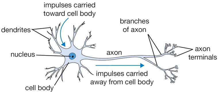
Mathematical Model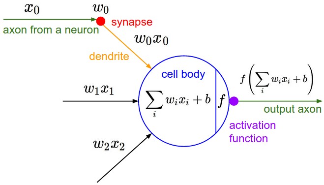
Simplified Neuron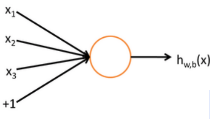

The neuron can be modeled as a binary logistic regression unit as in the last row of the table above. It can be further simplified as following functions,

• $\boldsymbol{x}$ is the inputs
• $\boldsymbol{w}$ is the weights
• $b$ is a bias term
• $h$ is a hidden layer function
• $f$ is a nonlinear activation function (sigmoid, tanh, etc.)

If we feed a vector of inputs through a bunch of logistic regression (sigmoid) functions, then we get a vector of outputs. The CS224N lecture note 3 section 1.2 have a complete derivation on multiple sigmoid units. But we don’t have to decide ahead of time what variables these logistic regressions are trying to predict! It is the loss function that will direct what the intermediate hidden variables should be, so as to do a good job at predicting the targets for the next layer, etc.

Forward Propagation in Matrix Notation¶

In a multilayer neural network, not only did we have multiple sigmoid units, but we also have more than one layer. Let's explicitly write down the signal transformation (aka forward propagation) from one layer to another referring to this network from Andrew's ML course.

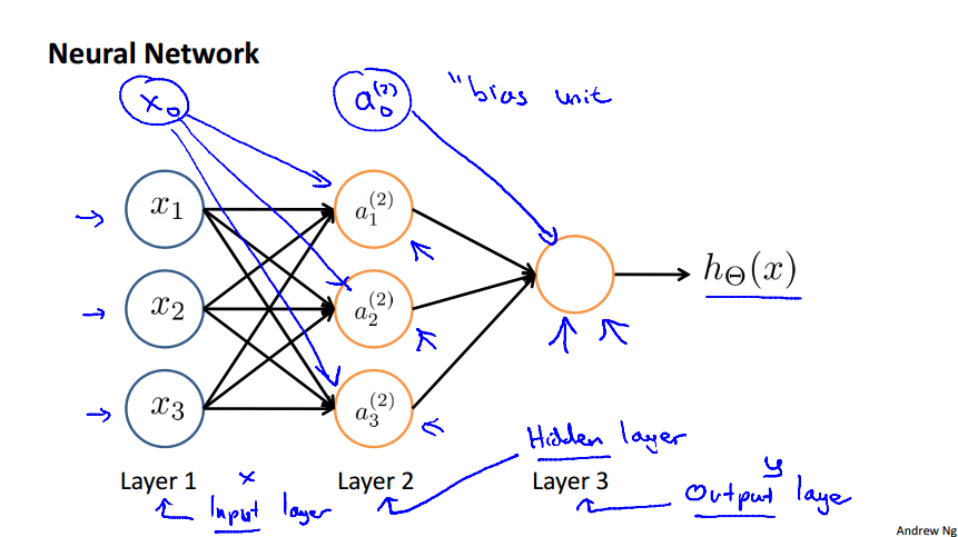
We will use the following notation convention

• $a^{(j)}_i$ to represent the "activation" of unit $i$ in layer $j$.
• $W^{(j)}$ to represent the matrix of weights controlling function mapping from layer $j$ to layer $j + 1$.

The value at each node can be calculated as

write the matrix $W^{(j)}$ explicity,

With the above form, we can use matrix notation as

We can see from above notations that if the network has $s_j$ units in layer $j$ and $s_{j+1}$ in layer $j + 1$, the matrix $W^{(j)}$ will be of dimention $s_{j+1} \times s_{j}+1$. It could be interpreted as "the dimention of $W^{(j)}$ is the number of nodes in the next layer (layer $j + 1$) $\times$ the number of nodes in the current layer $+$ 1.

the different is from how we denote the bias. The two are enssentially the same, but be cautions that the matrix dimentions are different.

Word Window Classification Using Neural Networks¶

From now on, let's switch the notation to cs224n so that we can derive the backpropagation algorithm for word window classification and get more intuition about the backprop. The drawing of the neural nets in cs224n for word window classification is less dynamic and slitly different from the drawing from Andrew's ML class. The figure from cs224n may be slightly confusing at first, but it is good to understand it from this word window classification application.

Forward propagation¶

Firstly, the goal of this classification task is to classify whether the center word is a location. Similar to word2vec, we will go over all positions in a corpus. But this time, it will be supervised and only some positions should get a high score.

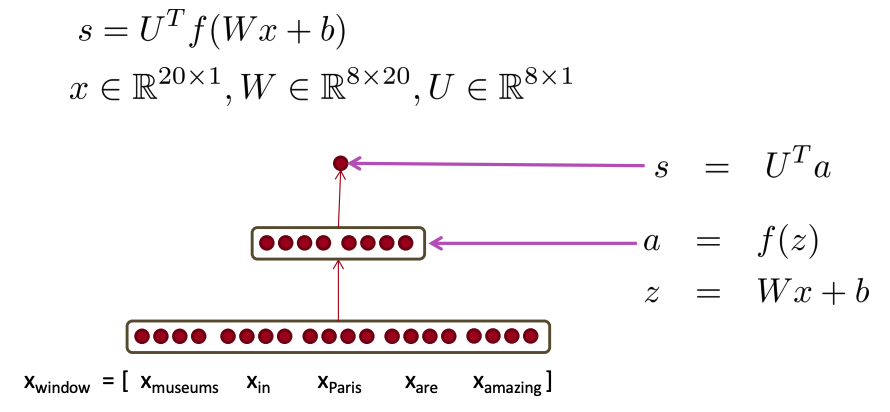
The figure above illustrate the feed-forward process. We use the method by Collobert & Weston (2008, 2011). An unnormalized score will be calculated from the activation $\boldsymbol{a} = [a_1, a_2, a_3, \cdots]^\mathsf{T}$.

We will use max-margin loss as our loss function. The training is essentially to find the optimal weights $W$ by minimize the max-margin loss

$s$ is the score of a window that have a location in the center. $s_c$ is the score of a window that doesn't have a location in the center. For full objective function: Sample several corrupt windows per true one. Sum over all training windows. It is similar to negative sampling in word2vec.

We will use gradient descent to update the parameter so as to minimize the loss function. The key is how to calculate the gradient with respect to the model parameters, namely $\nabla_{\theta} J(\theta)$. Here we use $\theta$ to represent the hyperthetic parameters, it can include the $W$ and other parameters of the model.

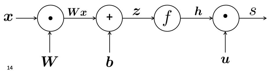
Gradients and Jacobians Matrix¶

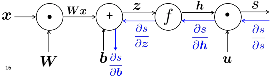
At first, let us layout the input and all the equations in this simple neural network.

To update the parameters in this model, namely $\boldsymbol{x}, \boldsymbol{W}, \boldsymbol{b}$, we would like to compute the derivitavies of $s$ with respect to all these parameters. We have to use the chain rule to compute it. What chain rule says is that we can compute the partial derivatives of each individual functions and then multiply them together to get the derivative with respect the specific variable. For example, $\frac{\partial s}{\partial \boldsymbol{b}}$ is computed as $\frac{\partial s}{\partial \boldsymbol{b}} = \frac{\partial s}{\partial \boldsymbol{h}} \cdot \frac{\partial \boldsymbol{h}}{\partial \boldsymbol{z}} \cdot \frac{\partial \boldsymbol{z}}{\partial \boldsymbol{b}}$. This seems very easy to understand, but when it comes to implemenation in vectorized format, it become confusing for those who doesn't work on matrix calculus for quite a while like me. I want to get the points straight here. What exactly is $\frac{\partial s}{\partial \boldsymbol{b}}$ and $\frac{\partial \boldsymbol{h}}{\partial \boldsymbol{z}}$. Note both $\boldsymbol{h}$ and $\boldsymbol{z}$ are vectors. To calculate these two gradient, simply remember the following two rules:

1. Given a function with 1 output and $n$ inputs $f(\boldsymbol{x}) = f(x_1, x_2, \cdots, x_n)$, it's gradient is a vector of partial derivatives with respect to each input (take the gradient element wise). $$ \frac{\partial f}{\partial \boldsymbol{x}} = \Bigg [ \frac{\partial f}{\partial x_1}, \frac{\partial f}{\partial x_2}, \cdots, \frac{\partial f}{\partial x_n}, \Bigg ] $$

2. Given a function with $m$ output and $n$ inputs $$ \boldsymbol{f}(\boldsymbol{x}) = \big [f_1(x_1, x_2, \cdots, x_n), \cdots, f_m(x_1, x_2, \cdots, x_n) \big ], $$ it's gradient is an $m \times n$ matrix of partial derivatives $(\frac{\partial \boldsymbol{f}}{\partial \boldsymbol{x}})_{ij} = \dfrac{\partial f_i}{\partial x_j}$. This matrix is also called Jacobian matrix.

Computing gradients with the chain rule¶

With these two rules we can calculate the partials. We will use $\frac{\partial s}{\partial \boldsymbol{b}}$ as an example.

• $\frac{\partial s}{\partial \boldsymbol{h}} = \frac{\partial}{\partial \boldsymbol{h}}(\boldsymbol{u}^{\mathsf{T}}\boldsymbol{h}) = \boldsymbol{u}^{\mathsf{T}}$

• $\frac{\partial \boldsymbol{h}}{\partial \boldsymbol{z}} = \frac{\partial}{\partial \boldsymbol{z}}(f(\boldsymbol{z})) = \begin{pmatrix} f'(z_1) & & 0 \\ & \ddots & \\ 0 & & f'(z_n) \end{pmatrix} = \mathrm{diag} (f' (\boldsymbol{z}))$

• $\frac{\partial \boldsymbol{z}}{\partial \boldsymbol{b}} = \frac{\partial}{\partial \boldsymbol{b}}(\boldsymbol{W}\boldsymbol{x} + \boldsymbol{b}) = \boldsymbol{I}$

Therefore,

Similarly we can calculate the partial with respect to $\boldsymbol{W}$ and $\boldsymbol{x}$. Since the top layer partials are already calculated, we can reuese the results. We denote those reusable partials as $\delta$ meaning local error signal.

Shape convention¶

What does the shape of the derivatives looks like in practice? How can we make the chain rule computation efficient? According to the aforementioned gradient calculation rules, $\frac{\partial s}{\partial \boldsymbol{W}}$ is a row vector. The chain rule gave

We know from Jacobians that $\frac{\partial\boldsymbol{z}}{\partial \boldsymbol{W}} = \frac{\partial}{\partial \boldsymbol{W}}(\boldsymbol{W}\boldsymbol{x} + \boldsymbol{b}) = \boldsymbol{x}^{\mathsf{T}}$. We may arrived the result that $\frac{\partial s}{\partial \boldsymbol{W}} = \boldsymbol{\delta} \ \boldsymbol{x}^{\mathsf{T}}$. This is actually not quite wirte. The correct form should be

Computation graphs and backpropagation¶

We have shown how to compute the partial derivatives using the chain rule. This is almost the backpropagation algorithm. If we want to add on to that and make the algorithm complete, the only thing we need is how to reuse gradient computed for higher layers. We leverage the computation graph to explain this. From the computation graph, you'll get the intuition of reusing the partial derivatives computed for higher layers in computing derivatives for lower layers so as to minimize computation.

We represent our neural net equations as a computation graph as following:

• source nodes represent inputs
• interior nodes represent operations
• edges pass along result of the operation

When following computation order to carry out the computations from inputs, it is forward propagation. Backpropagation is to pass along gradients backwards. This can be illustrated in the following computation graph.

The partial derivative with respect to a parameter reflect how changing the parameter would effect the output value. The output value in the backprop is usually a loss function (or error). Intuitively, you can see backprop is push the error back to the lower layer through a bunch of operation nodes, the arrived error is a measure of the error at that particular layer, training is try to reduce this backprop-ed error by adjusting the local parameters, the effect of reducing the local error will be forward propagated to the output, the error at the output should also reduced. We use gradient descent to make this process to converge as soon as possible.

To understand it better, let's look at a single node.

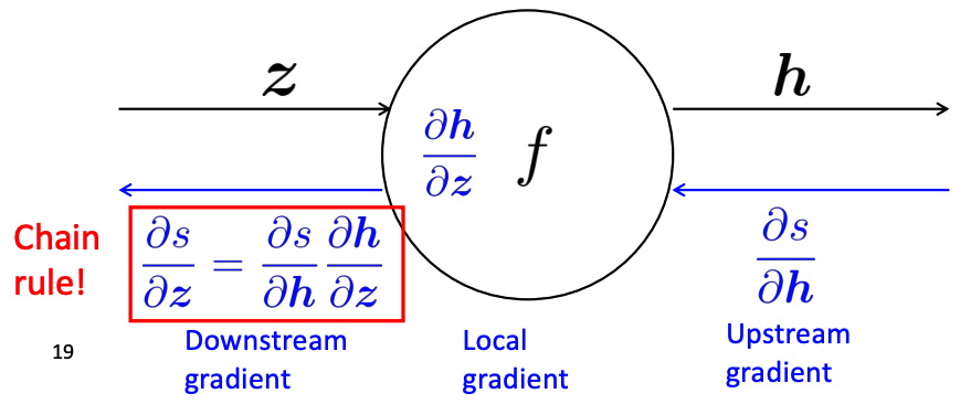
We define "local gradient" for each node as the gradient of it's output with respect to it's input. By chain rule, the downstream gradient is equal to the multiplication of the upstream gradient and the local gradient. When having multipe local gradients, they are pushed back to each input using chain rule. CS224N lecture 4 slides have step by step example of backprop. From the example, we can got some intuitions about some nodes' effects. For example, when push back gradients along outward branches from a single node, the gradients should be sumed up; "+" node distributes the upstream gradient to each summand; "max" node simply routes the upstream gradients.

When update gradient with backprop, you should compute all the gradients at once. With this computation graph notion, following routine captures the gist of backprop in a very decent manner.

1. Fprop: visit nodes in topological sorted order
2. Compute value of node given predecessors
3. Bprop:
4. initialize output gradient = 1
5. visit nodes in reverse order:
   • Compute gradient wrt each node using gradient wrt successors
   • $\{y_1, y_2, \cdots, y_2\} = \mathrm{successors\ of\ } x$

$$\begin{equation*}\frac{\partial z}{\partial \boldsymbol{x}} = \sum_{i=i}^n \frac{\partial z}{\partial y_i} \frac{\partial y_i}{\partial x} \end{equation*}$$

If done correctly, the big $O$ complexity of forward propagation and backpropagation is the same.

Automatic differentiation¶

The gradient computation can be automatically inferred from the symbolic expression of the fprop. but this is not commonly used in practice. Each node type needs to know how to compute its output and how to compute the gradient wrt its inputs given the gradient wrt its output. Modern DL frameworks (Tensorflow, PyTorch, etc.) do backpropagation for you but mainly leave layer/node writer to hand-calculate the local derivative. Following is a simple demo of how to implement forward propagation and backpropagation.

class MultiplyGate(object):
    def forward(x, y):
        z = x * y
        self.x = x # must keep these around!
        self.y = y
        return z

    def backword(dz):
        dx = self.y * dz # [dz/dx * dL/dz]
        dy = self.x * dz # [dz/dy * dL/dz]
        return [dx, dy]

1. nonlinear activation functions: sigmoid, tanh, hard tanh, ReLU
2. Learning rates: start 0.001. power of 10. halve the learning rate every k epochs. formula: $lr = lr_0 e^{-k t}$ for each epoch $t$

Regularization¶

LFD

1. starting point: L2 regularization

Part 3 Language Model and RNN¶

n-gram¶

• assumption: $\boldsymbol{x}^{(t+1)}$ depends only on previous $n-1$ words.
• Sparsity problem, --> backoff (n-1)-gram
• practically, n has to be less than 5.

Neural language model¶

• fixed-window neural language model
• Recurrent Neural Network