Machine Learning (Coursera)
Week 1 Introduction
Quote
Machine Learning is a field of study that gives computers the ability to learn without being explicitly programmed. -- Arthur Samuel (1959)
Quote
A computer program is said to learn from experience E with respect to some task T and some performance measure P, if its performance on T, as measured by P, improves with experience E. -- Tom Mitchell (1998)
- Well-posed Learning Problem
- Experience E
- Task T
- Performance P
- Supervised learning: give the "right answer" of existing
- Unsupervised learning
- Reinforcement learning
- Recommendation system
-
Regression V.S. classification
- Regression, predict a continuous value across range
- a function of independent variable
- Classification, predict a discrete value
- Regression, predict a continuous value across range
Cost Function
- Cost function (squared error function)
- Goal
-
Some Intuitions
- when the sample is
{1, 1}, {2, 2}, and {3, 3}. h_\theta(x) = x, (\theta_0 = 0, \theta_1 = 1), we can calculate J(\theta_0, \theta_1) = 0. - when the sample is
{1, 1}, {2, 2}, and {3, 3}. h_\theta(x) = 0.5 x, (\theta_0 = 0, \theta_1 = 0.5), we can calculate J(\theta_1) = \frac{3.5}{6}. - we can plot J(\theta_1) vs. \theta_1, the function plotted would be a quadratic curve.
- when the sample is
Cost Function Intuition I
- Andrew plot the hypothesis \textstyle h_\theta(x) and the cost function \textstyle {J(\theta_1)}(setting \theta_0 = 0), The function \textstyle J(\theta_1) is a curve have a minimum value.
Cost Function Intuition II
-
The plot of h(x) and J(\theta_0, \theta_1) show that J(\theta_0, \theta_1) has to be contour plot.
-
Our goal is to \min_{\theta_0, \theta_1}J(\theta_0, \theta_1)
To summarize, in this lecture, we formulate the hypothesis function and defined the cost function. We also plotted them to get some insight into the two functions. The machine learning problem we learn from this lecture is a minimization problem. Given a hypothesis, we looking for the \theta_0 and \theta_1 which minimize the cost function. Then we solve the problem. We use the Gradient Descent algorithm to search this minimum value.
Gradient Descent
- It could solve general minimization problems
- Given function J(\theta_0, \theta_1)
- Objective: \min_{\theta_0, \theta_1}J(\theta_0, \theta_1)
Gradient Descent Algorithm
- Start with some \theta_0, \theta_1
- Keep changing \theta_0, \theta_1 to reduce J(\theta_0, \theta_1)
- Simultianeously update: \theta_j := \theta_j - \alpha \frac{\partial }{\partial \theta_j}J(\theta_0, \theta_1), for ( j = 0, j = 1)
- Keep changing \theta_0, \theta_1 to reduce J(\theta_0, \theta_1)
- Untill we hopefully end up at the minimum.(convergence)
- Question: How to implement the algorithm.
Gradient Descent Intuition
- learning rate
- don't have to adjust the learning rate
- derivative
- would reduce automatically
Gradient Descent and Linear Regression
- Take the linear regression cost function and apply gradient descent algorithm.
- Model: h_\theta(x) = \theta_0 + \theta_1x
- Cost function: J(\theta_0, \theta_1) = \frac{1}{2m}\sum_{i=1}^{m}(h_\theta(x^{(i)}) - y^{(i)})^2
- Gradient Descent in Linear Regression.
repeat \begin{Bmatrix} \theta_0 := \theta_0 - \alpha \frac{1}{m} \sum_{i = 1}^{m}(h_\theta(x^{(i)}) - y^{(i)}) \\ \theta_1 := \theta_1 - \alpha \frac{1}{m} \sum_{i = 1}^{m}(h_\theta(x^{(i)}) - y^{(i)}) x^{(i)} \end{Bmatrix} simultaneously.
- The linear regression cost function is always a convex function - always has a single minimum (bowl Shaped).
Linear Algebra Review
- Not commutative: A x B != B x A except that matrix B is identity matrix.
- Associativity: (A x B) x C = A x (B x C)
- Identity Matrix:
- Any matrix A which can be multiplied by an identity matrix gives you matrix A back
- I[m, m] x A[m, n] = A[m, n]
- A[m, n] x I[n, n] = A[m,n]
- Inverse
- Multiplicative inverse(reciprocal): a number multiply it by to get the identify element. i.e. if you have
x,x * 1/x = 1. - Additive inverse: -3 is 3's additive inverse.
- Multiplicative inverse(reciprocal): a number multiply it by to get the identify element. i.e. if you have
- Matrix inverse
- A \cdot A^{-1} = I
- Only square matrix, but not all square matrix have an inverse.
- singularity
- If A is all zeros then there is no inverse matrix
- Some others don't, intuition should be matrices that don't have an inverse are a singular matrix or a degenerate matrix (i.e. when it's too close to 0)
- So if all the values of a matrix reach zero, this can be described as reaching singularity
Week 2 Multiple features(variables) linear regression
- From feature x^{(i)}to features x_j^{(i)}, means the jth feature element of the ith feature vector.
- Hypothesis becomes: \textstyle h_\theta(x) = \theta^{T}x = \theta_0x_0 + \theta_1x_1 + ... + \theta_nx_n.
- Cost Function: J(\theta_0, \theta_1, ..., \theta_n) = \frac{1}{2m}\sum_{i=1}^{m}(h_\theta(x^{(i)}) - y^{(i)})^2
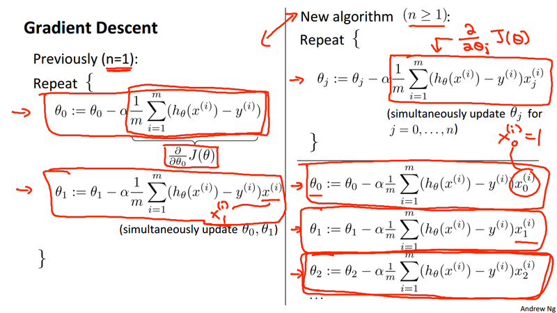
- Gradient descent: \theta_j := \theta_j - \alpha \frac{\partial }{\partial \theta_j}J(\theta_0, \theta_1, ..., \theta_n), simultaneously update for every j = 0, 1, 2, ..., n.
- Compare of Gradient descent for multiple variables:
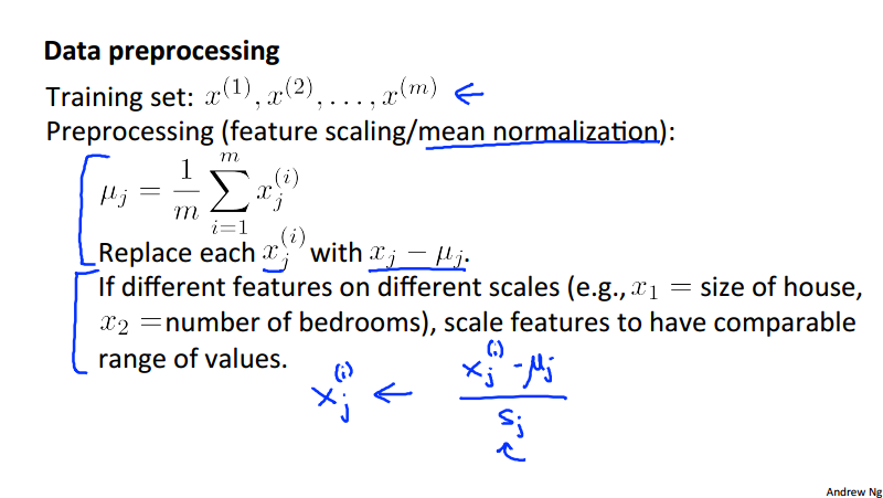
Feature scaling
One of the idea to improve the result in gradient descent is to make different features in the same scale, i.e. -1 \leq x_i \leq 1 range .
For example, in the housing price prediction problem, we have to make the size of the house (0-2000 square feet), and the number of rooms in the house (1-5 rooms) in the same scale. We do this by the method of mean normalization.
- Mean normalization Replace x_i with x_i - \mu_i to make features have approximately zero mean (Do not apply to x_0 = 1)
- E.g. x_1 = \frac{size - 1000}{2000}, x_2 = \frac{\#rooms - 2}{5(range)} to make -0.5 \le x_1 \le 0.5, -0.5 \le x_2 \le 0.5,
Learning rate
Another idea to improve the gradient descent algorithm is to select the learning rate \alpha to make the algorithm works correctly.
- Convergence test: we can declare convergence if J(\theta) decreases by less than 10^{-3} in one iteration.
For sufficient small \alpha, J(\theta) should decrease on every iteration, but if \alpha is too small, gradient descent can be slow to converge. If \alpha is too large: J(\theta) may not decrease on every iteration, may not converge.
- Rule of Thumb: to choose \alpha, try these numbers
..., 0.001, 0.003, 0.01, 0.03, 0.1, 0.3, 1, ...
Polynomial Regression
In the house price prediction proble. if two features selected are frontage and depth. we can also take the polynomial problem, take the area as a single feature, thusly reduce the problem to a linear regression. We could even take the higher polynomials of the size feature, like second order, third order, and so on. for example,
h_\theta = \theta_0 + \theta_1x_1 + \theta_2x_2 + \theta_3x_3 = \theta_0 + \theta_1(size) + \theta_2(size)^2 + \theta_3(size)^3
In this case, the polynomial regression problem will fit in a curve instead of a line.
Normal Equation
Normal Equation: Method to solve for θ analytically. The intuition comes that we can mathematically sovle \frac{\partial}{\partial\theta_j}J(\Theta) = 0 for \theta_0, \theta_1, \dots, \theta_n, given the J(\Theta).
The equation to get the value of \Theta is \Theta = (X^TX)^{-1}X^Ty, in Octave, you can calculate by the command pinv(X'*X)*X'*y), pay attention to the dimention of the the matrix X and y.
Normal equation and non-invertibility
TBD
Week 3 Logistic regression model
Classification problem
- Email: spam / Not spam?
- Tumor: Malignant / Benign?
-
Example:
-
y is either 0 or 1
- 0: Negative class
- 1: Positive class.
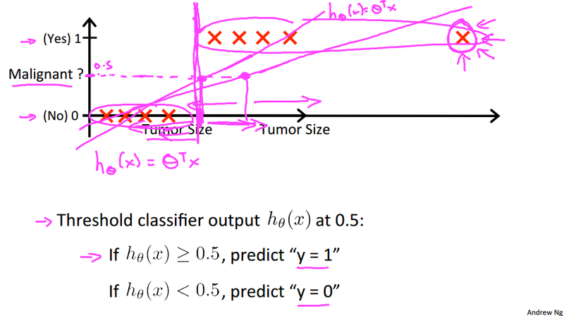
- With linear regression and a threshold value, we can use linear regression to solve classification problem.
- However linear regression could result in the case when h_\theta(x) is > 1 or < 0.
- Need a different method which will make 0 \le h_\theta(x) \le 1. This is why logistic regression comes in.
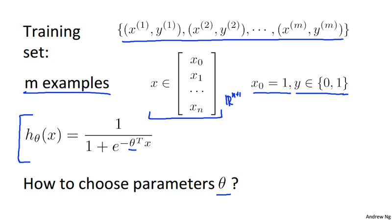
Hypothesis representation
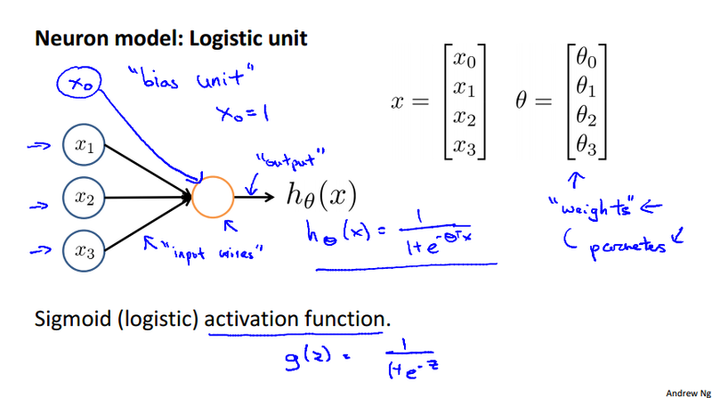
Because we want to have 0 \le h_\theta(x) \le 1, the domain of sigmoid function is in the range. From linear regression h_\theta(x) = \theta^Tx, we can have h_\theta(x) for logistic regression:
g_\theta(z) = \frac{1}{1 + e^{-z}} is Sigmoid function, also called logistic function. now in logistic regress model, we can write
Interpretation
- Logistic regression model h_\theta(x) = \frac{1}{1 + e^{-\theta^Tx}}, is the estimated probability that y = 1 on input x. i.e. h_\theta(x) = 0.7 tell patient that 70% chance of tumore being malignant.
- h_\theta(x) = P(y = 1|x;\theta),
- P(y=0|x; \theta) + P(y=1|x;\theta) = 1
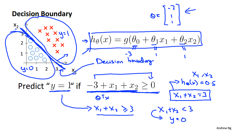
Logistic regression decision boundary
- Gives a better sense of what the hypothesis function is computing
- Better understanding of what the hypothesis function looks like
- One way of using the sigmoid function is:
- When the probability of y being 1 is greater than 0.5 then we can predict y = 1
- Else we predict y = 0
- When is it exactly that h_\theta(x) is greater than 0.5?
- Look at sigmoid function
- g(z) is greater than or equal to 0.5 when z is greater than or equal to 0.
- So if z is positive, g(z) is greater than 0.5
- z = (\theta^T x)
- So when
- \theta^T x >= 0
- Then h_\theta(x) >= 0.5
- Look at sigmoid function
- So what we've shown is that the hypothesis predicts y = 1 when \theta^T x >= 0
- The corollary of that when \theta^T x <= 0 then the hypothesis predicts y = 0
- Let's use this to better understand how the hypothesis makes its predictions
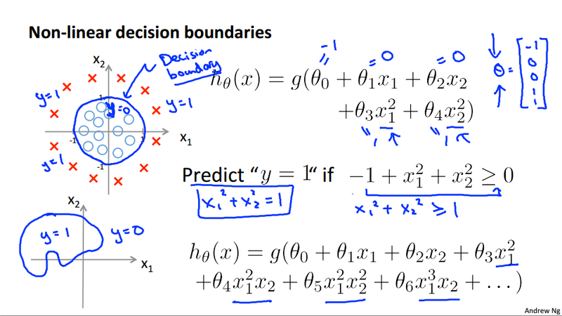
- Linear Decision boundary and non-linear decision boundary
Logistic regression cost function
Problem description
Logistic Regression Cost Function
Out goal to solve a logistic regression problem is to reduce the cost incurred when predict wrong result. In linear regression, we minimize the cost function with respect to vector \theta. Generally, we can think the cost function as a penalty of the incorrect classification. It is a qualitative measure of such penalty. For example, we use the squared error cost function in linear regression:
In logistic regression, the h_\theta(x) is a much complex function, so the cost function J(\theta) used in linear regression will be a non-convex function in logisitic regress. This will produce a hard problem to solve logistic problems numerically. So we define a convex logistic regression cost function
It is the logistic regression cost function, it can be interpreted as the penalty the algorithm pays.
We can plot the function as following:
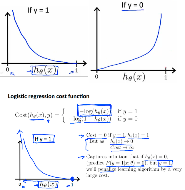
Some intuition/properties about the simplified logistic regression cost function:
- X axis is what we predict
- Y axis is the cost associated with that prediction.
- If y = 1, and h_\theta(x) = 1, hypothesis predicts exactly 1 (exactly correct) then cost corresponds to 0 (no cost for correct predict)
- If y = 1, and h_\theta(x) = 0, predict P(y = 1|x; \theta) = 0, this is wrong, and it penalized with a massive cost (the cost approach positive infinity).
- Similar reasoning holds for y = 0.
Gradient descent and cost function
We can neatly write the logistic regression function in the following format:
We can take this cost function and obtained the logistic regression cost function J(\theta):
Why do we chose this function when other cost functions exist?
- This cost function can be derived from statistics using the principle of maximum likelihood estimation.
- Note this does mean there's an underlying Gaussian assumption relating to the distribution of features.
- Also has the nice property that it's convex function.
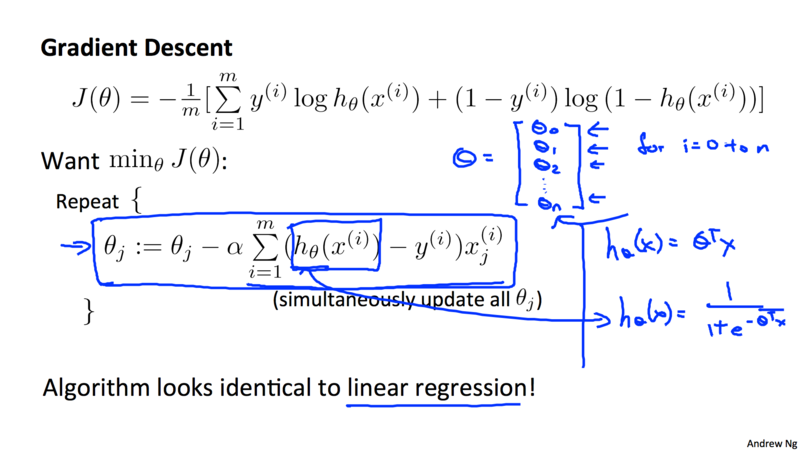
Gradient Descent for logistic regression
The algorithm looks identical to linear regression except the hypothesis function is Sigmoid function and not linear any more.
Advanced Optimization
Beside gradient descent algorithm, there are many other optimization algorithm such as conjugate gradient, BFGS, and L-BFGS, can minimization the cost function for solving logistic regression problem. Most of those advanced algorithms are more efficient to compute, you don't have to select the convergent rate \alpha.
Here is one function in Octave library, possibly also in Matlab, can be used for finding the \theta
Function fminunc()
Octave have a function fminunc().^1 To use it, we should first call optimset(). There is three steps we need to take care to solve optimization problem using these functions
- calculate the cost function J(\theta)
- calculate the gradient functions \frac{\partial}{\partial\theta_j}J(\theta)
- give initial \theta value
-
call the function
optimset()andfminunc()as followingfunction [jVal, gradient] = costFunction(theta) jVal = (theta(1)-5)^2 + (theta(2)-5)^2; gradient = zeros(2,1); gradient(1) = 2*(theta(1)-5); gradient(2) = 2*(theta(2)-5); options = optimset(‘GradObj’, ‘on’, ‘MaxIter’, ‘100’); initialTheta = zeros(2,1); [optTheta, functionVal, exitFlag] = fminunc(@costFunction, initialTheta, options); -
Note we have
n+1parameters, we implement the code in the following way.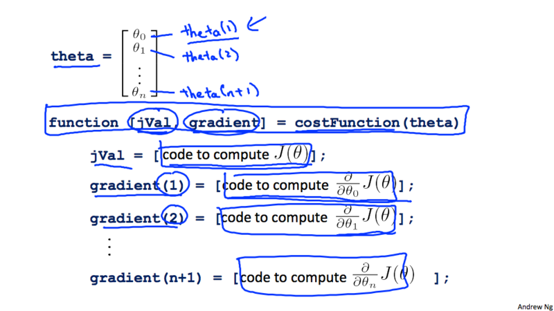
Multiclass classification
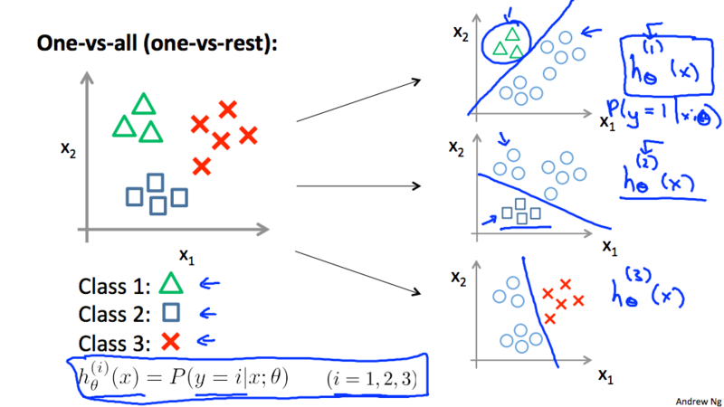
- Train a logistic regression classifier h_{\theta}^{(i)}(x) for each class i to predict the probability that y = i.
- On a new input x, to make a prediction, pick the class i that maximize the h, \operatorname*{argmax}_i h_{\theta}^{(i)}(x)
Regularization
Overfitting
If we have too many features, the learned hypothesis may fit the training set very well ( J(\theta) \approx 0 ), but fail to generalize to new examples (predict prices on new examples).
Address overfitting problems
- Reduce the number of features
- Manually select what features to keep
- feature selection algorithm
- Regularization
- Keep all the features, reduce the value of the parameter \theta_j.
- work well when we have a lot of data when each of the features contribute to the algorithm a bit to predict y.
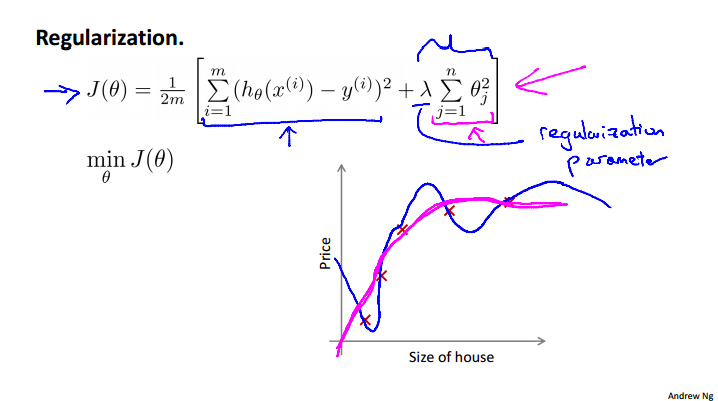
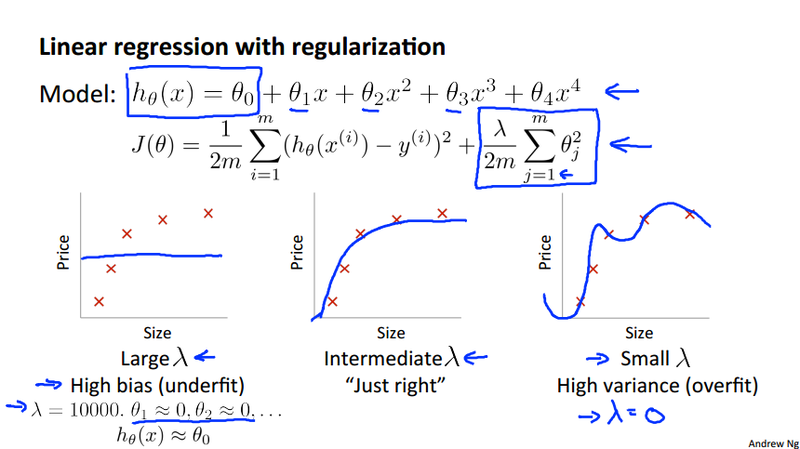
Regularization Intuition
To penalize the higher order of polynomial by adding extra terms of high coefficient for \theta^n terms. i.e. from the cost function minimization problem, J(\theta) = \frac{1}{2m}\sum_{i=1}^{m}(h_\theta(x^{(i)}) - y^{(i)})^2, we can instead use the regularized form J(\theta) = \frac{1}{2m}\sum_{i=1}^{m}(h_\theta(x^{(i)}) - y^{(i)})^2 + \lambda\sum_{j = 1}^{n}\theta_j^2. Small values for parameters \theta_j will make "Simpler" hypothesis and Less prone to overfitting. Please note that the \theta_0 is excluded from the regularization term \lambda\sum_{n = 1}^{n}\theta_j^2.
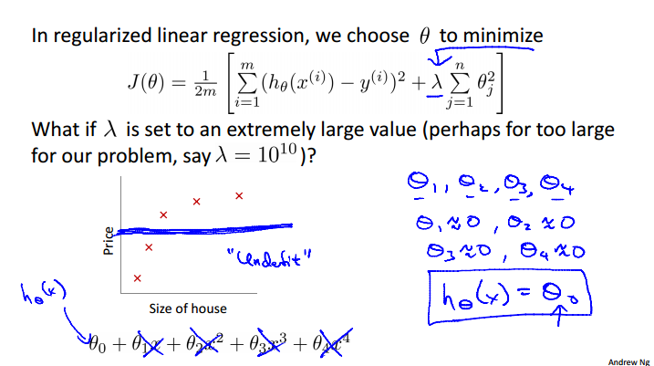
Regularized linear regression
Gradient Descent:
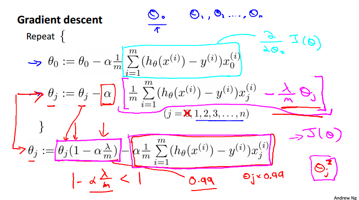
- We don't regularize \theta_0, so we explicitly update it in the formula and it is the same with the non-regularized linear regression gradient descent. All other \theta_j, j = 1, ..., n will update differently.
Regularized logistic regression
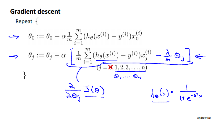
- Doesn't regularize the \theta_0
- The cost function is different from the linear regression
Advanced optimization
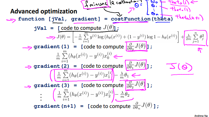
- Add the regularized term in the cost function and gradient calculation
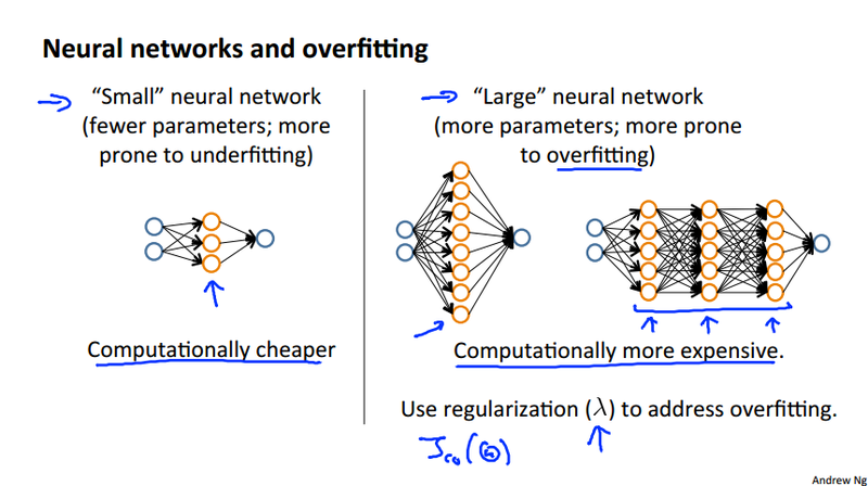
Week 4 Neural networks model
Neural Networks is originated when people try to mimic the functionality of brain by an algorithm.
Model representation
In an artificial neural network, a neuron is a logistic unit that
- Feed input via input wires
- Logistic unit does the computation
- Sends output down output wires
The logistic computation is just like our previous logistic regression hypothesis calculation.
Neural Network
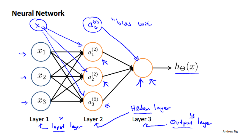
Use the following notation convention:
- a_i^{(j)} to represent the \"activation\" of unit i in layer j
- \Theta^{(j)} to represent the matrix of weights controlling function mapping from layer j to layer j+1
The value at each node can be calculated as
If the network has s_j units in layer j, s_{j+1} units in layer j+1, then \Theta^{(j)} will be of dimension s_{j+1} \times (s_j + 1). It could be interpreted as "the dimension of \Theta^{(j)} is number of nodes in the next layer \times the current layer's node + 1".
Forward propagation implementation
By defining z_1^{(2)}, z_1^{(2)}, and z_1^{(2)}, we could obtain a_1^{(2)} = g(z_1^{(2)}), where z_1^{(2)} = \theta_{10}^{(1)}x_0 + \theta_{11}^{(1)}x_1 + \theta_{12}^{(1)}x_2 + \theta_{13}^{(1)}x_3. To make it more compact, we define x = \left[ \begin{array}{c} x_0 \\ x_1 \\ x_2 \\ x_3 \end{array} \right] and z^{(2)} = \left[ \begin{array}{c}z_1^{(2)} \\ z_2^{(2)} \\ z_3^{(2)} \end{array} \right], so we have reached the following vectorized implementation of neural network. It is also called forward propagation algorithm.
Input: x
Forward Propagation Algorithm:
z^{(2)} = \Theta^{(1)}x a^{(2)} = g(z^{(2)}) and a_0^{(2)} =1. z^{(3)} = \Theta^{(3)}a^{(2)} h_{\Theta}(x) = a^{(3)} = g(z^{(3)})
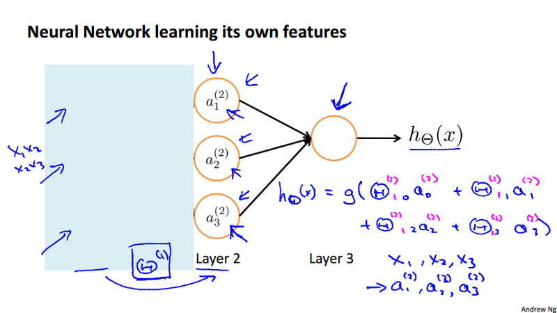
Learning its own features
What neural network is doing is it just like logistic regression, rather than using hte original feature, x_1, x_2, x_3, it use new feature a_1^{(2)}, a_1^{(2)}, a_1^{(2)}. Those new feature are learned from the original input x_1, x_2, x_3.
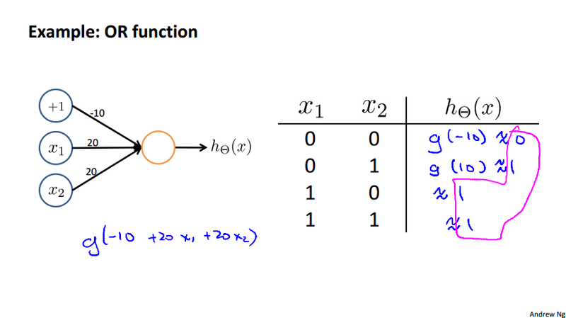
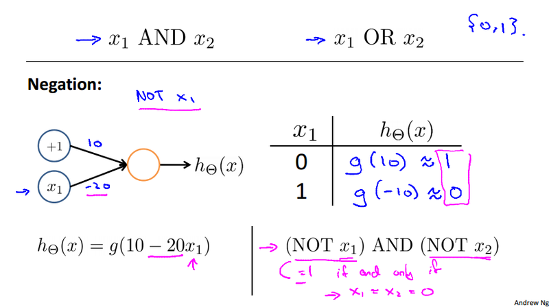
XNOR example
We calculate a Non-linear classification example: XOR/XNOR, where x_1 and x_2 are binary 0 or 1. y = x_1 \text{ XNOR } x_2 = \text{ NOT } (x_1 \text{ XOR } x_2). But those are all build on the basic non-linear operation AND, OR, and NOT.
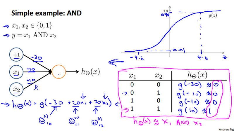
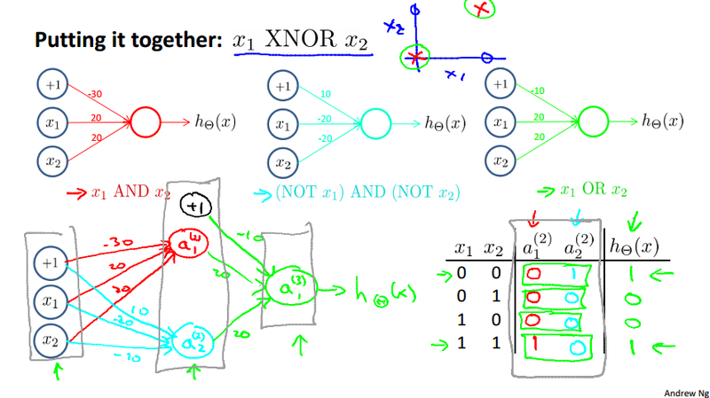
Don't worry about how we get the \theta. This example just to give some intuitions of how neural network problem can be solved.
Multiclass classification
Suppose our algorithm is to recognize pedestrian, car, motorbike or truck, we need to build a neural network with four output units. We could use a vector to do this When image is a pedestrian get [1,0,0,0] and so on.
- 1 is 0/1 pedestrain
- 2 is 0/1 car
- 3 is 0/1 motorcycle
- 4 is 0/1 truck
Just like one vs. all classifier described earlier. here we have four logistic regression classifiers
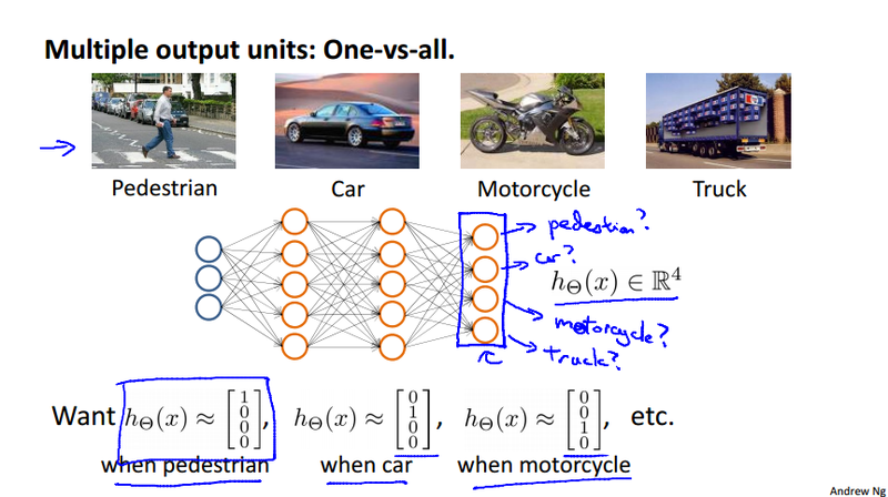
Contrast to the previous notation we wrote y as an integer {1, 2, 3, 4} to represent four classes. Now we use the following notation to represent y^{(i)} as one of \left[ \begin{array}{c} 1 \\ 0 \\ 0 \\ 0 \end{array} \right], \left[ \begin{array}{c} 0 \\ 1 \\ 0 \\ 0 \end{array} \right], \left[ \begin{array}{c} 0 \\ 0 \\ 1 \\ 0 \end{array} \right], \left[ \begin{array}{c} 0 \\ 0 \\ 0 \\ 1 \end{array} \right].
Week 5 Neural networks learning
Neural network classification
The cost function of neural network would be a generalized form of the regularized logistic regression cost function as shown below.
Cost Function
Logistic regression
Neural Network
We have the hypothesis in the K dimensional Euclidean space, denoted as h_{\Theta}(x) \in \mathbb{R}^K, K is the number of output units. (h_{\Theta}(x))_i = i^{th} output.
Noticed that all the summation is start from 1 not 0. For example, the index k and j. Because we don't regularize the bias unit which is with subscript 0.
Gradient computation
We have the cost function for the neural network. Next step we need to calculate the gradient of the cost function. As we can see that the cost function is too complicated to derive its gradient. Here we will use back propagation method to calculate the partial derivative. Before dive into the details of the back propagation, we need to summarize some of the ideas we had for the neural network so far.
Forward propagation
- Forward propagation takes initial input into that neural network and pushes the input through the neural network
- It leads to the generation of an output hypothesis, which may be a single real number, but can be a vector.
Back propagation
The appearance of the back propagation algorithm isn't very natural. Instead, it is a very smart way to solve the optimization problem in neural network. Because it is difficult to follow the method we used in linear regression or logistic regression to analytically get the derivative of the cost function. Back propagation come to help solving the optimization problem numerically.
To compute the partial derivative \frac{\partial}{\partial\Theta_{i,j}^{(l)}}J(\Theta) (the gradient of cost function in neural network), thus allow us to find the parameter \Theta that minimize the cost J(\Theta) (using gradient descent or advanced optimization algorithm), which will result in a hypothesis with parameters learn from the existing data.
How to derive the back-prop
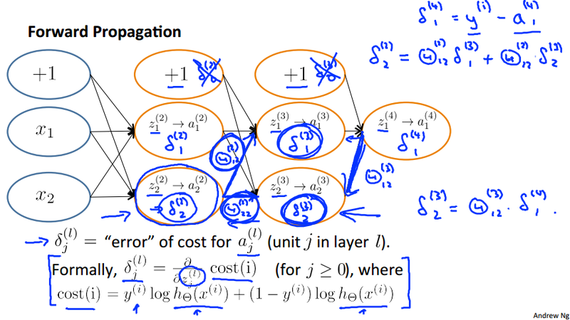
- We define \delta_{j}^{(l)} = \"error\" of node j in layer l
- We calculate \delta^{(L)} = a^{(L)} - y, which is the vector of errors defined above at last layer L. Note \delta^{(L)} is vectorized representation of \delta_{j}^{(l)}. So our "error values" for the last layer are simply the differences of our actual results a^{(L)} in the last layer and the correct outputs in y.
- To get the delta values of the layers before the last layer, we can use an equation that steps us back from right to left, thereby back propagate, by \delta^{(l)} = ((\Theta^{(l)})^T\delta^{(l+1)}).*g'(z^{(l)}). It can be interpreted as the error value of layer l are calculated by multiplying the error values in the next layer with theta matrix of layer l. We then element wise multiply that with the derivative of the activation function a^{(l)} = g(z^{(l)}), namely g'(z^{(l)}) = a^{(l)}.*(1-a^{(l)}). The derivation of this deviative can be found at the course wiki.
- Partial derivative. With all the calculated \delta^{(l)} values, We can compute our partial derivative terms by multiplying our activation values and our error values for each training example t, \dfrac{\partial}{\partial \Theta_{i,j}^{(l)}}J(\Theta) = \frac{1}{m}\sum_{t=1}^m a_j^{(t)(l)} {\delta}_i^{(t)(l+1)}. This is ignoring regularization terms.
- Notations:
- t is the index of the training examples, we have total of m samples.
- l is the layer, we have total layer of L.
- i is the error affected node in the target layer, layer l+1.
- j is the node in the current layer l.
- \delta^{(l+1)} and \ a^{(l+1)} are vectors with s_{l+1} elements. Similarly, \ a^{(l)} is a vector with s_{l} elements. Multiplying them produces a matrix that is s_{l+1} by s_{l} which is the same dimension as \Theta^{(l)}. That is, the process produces a gradient term for every element in \Theta^{(l)}. |
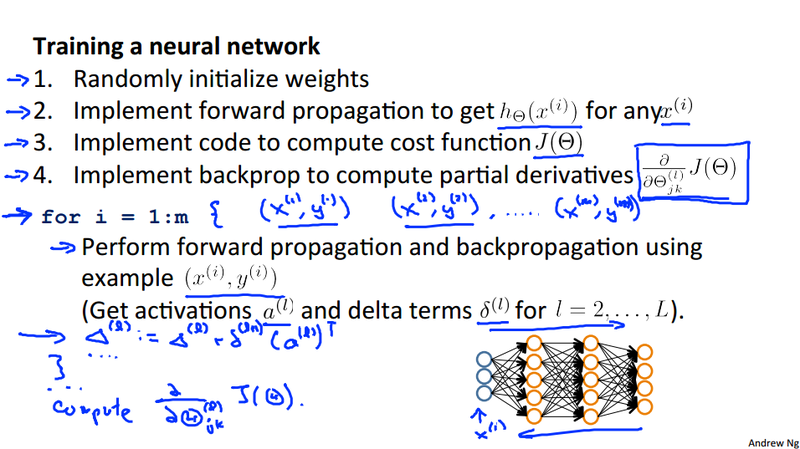
Backpropagation Algorithm
- Given training set \lbrace (x^{(1)}, y^{(1)}) \cdots (x^{(m)}, y^{(m)})\rbrace
- Set \Delta^{(l)}_{i,j} := 0 for all (l,i,j)
- For training example t = 1 to m:
- Set a^{(1)} := x^{(t)}
- Perform forward propagation to compute a^{(l)} for l = 2,3,\dots ,L
- Using y^{(t)}, compute \delta^{(L)} = a^{(L)} - y^{(t)}
- Compute \delta^{(L-1)}, \delta^{(L-2)},\dots,\delta^{(2)} using \delta^{(l)} = ((\Theta^{(l)})^T \delta^{(l+1)})\ .*\ a^{(l)}\ .*\ (1 - a^{(l)})
- \Delta^{(l)}_{i,j} := \Delta^{(l)}_{i,j} + a_j^{(l)} \delta_i^{(l+1)} or with vectorization, \Delta^{(l)} := \Delta^{(l)} + \delta^{(l+1)}(a^{(l)})^T (programmatic calculation of \frac{1}{m}\sum_{t=1}^m a_j^{(t)(l)} {\delta}_i^{(t)(l+1)})
- D^{(l)}_{i,j} := \dfrac{1}{m}\left(\Delta^{(l)}_{i,j} + \lambda\Theta^{(l)}_{i,j}\right) If j \neq 0 (NOTE: Typo in lecture slide omits outside parentheses. This version is correct.)
- D^{(l)}_{i,j} := \dfrac{1}{m}\Delta^{(l)}_{i,j} If j = 0
The capital-delta matrix is used as an \"accumulator\" to add up our values as we go along and eventually compute our partial derivative.
The actual proof is quite involved, but, the D^{(l)}_{i,j} terms are the partial derivatives and the results we are looking for: D_{i,j}^{(l)} = \dfrac{\partial J(\Theta)}{\partial \Theta_{i,j}^{(l)}}.
Math representation
- There is a \Theta matrix for each layer in the network
- This has each node in layer l as one dimension and each node in l+1 as the other dimension
- Similarly, there is going to be a \Delta matrix for each layer
- This has each node as one dimension and each training data example as the other
A high level description
- Back propagation basically takes the output you got from your network, compares it to the real value (y) and calculates how wrong the network was (i.e. how wrong the parameters were)
- It then, using the error you\'ve just calculated, back-calculates the error associated with each unit from right to left.
- This goes on until you reach the input layer (where obviously there is no error, as the activation is the input)
- These \"error\" measurements for each unit can be used to calculate the partial derivatives
- Partial derivatives are the bomb, because gradient descent needs them to minimize the cost function
- We use the partial derivatives with gradient descent to try minimize the cost function and update all the \Theta values
- This repeats until gradient descent reports convergence
What we need to watch out?
- We don\'t have \delta^{(1)} because we have all x, it is zero.
- We don\'t calculate the bias node.
Backpropagation Intuition
Backpropagation very similar to the forward propagation, we can use a example to calculate the \lambda_i^{(\ell)} or the z^{(\ell)} as bellow. To further understand the algorithm, refer to the code in assignment 4.
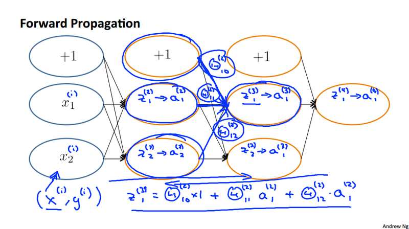
As it is shown in the slide, z_1^{(2)} is calculate by multiply the corresponding \Theta^{(2)}_{ij} value. the index i is the same as in z_i^{(2)}. The index j means the jth node in the previous layer.
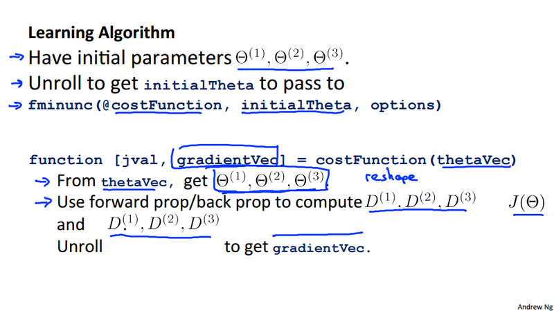
Unrolling parameters
With neural networks, we are working with sets of matrices: \Theta^{(1)}, \Theta^{(2)}, \Theta^{(3)}, \dots. D^{(1)}, D^{(1)}, D^{(3)}, \dots
In order to use optimizing functions such as "fminunc()", we will want to "unroll" all the elements and put them into one long vector
# unroll the matrices
thetaVector = [ Theta1(:); Theta2(:); Theta3(:); ]
deltaVector = [ D1(:); D2(:); D3(:) ]
If the dimensions of Theta1 is 10x11, Theta2 is 10x11 and Theta3 is 1x11, then we can get back our original matrices from the "unrolled" versions as follows
# using reshape function to build matrix from vectors
Theta1 = reshape(thetaVector(1:110),10,11)
Theta2 = reshape(thetaVector(111:220),10,11)
Theta3 = reshape(thetaVector(221:231),1,11)
In Octave, if we want to implement the back propagation algorithm, we have to do the unrolling and reshaping back and forth in order to calculate the gradientVec. Notice that the last two lines are shifted in the picture, it should read "Use forward propagation and back propagation to compute D^{(1)}, D^{(1)}, D^{(3)} and J(\Theta). Unroll D^{(1)}, D^{(1)}, D^{(3)} to get gradientVec.
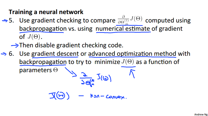
Gradient Checking
To ensure a bug free back propagation implementation, one method we can use is gradient checking. It is a way of numerically estimate the gradient value in each computation point. It works as a reference value to check the back propagation is correct.
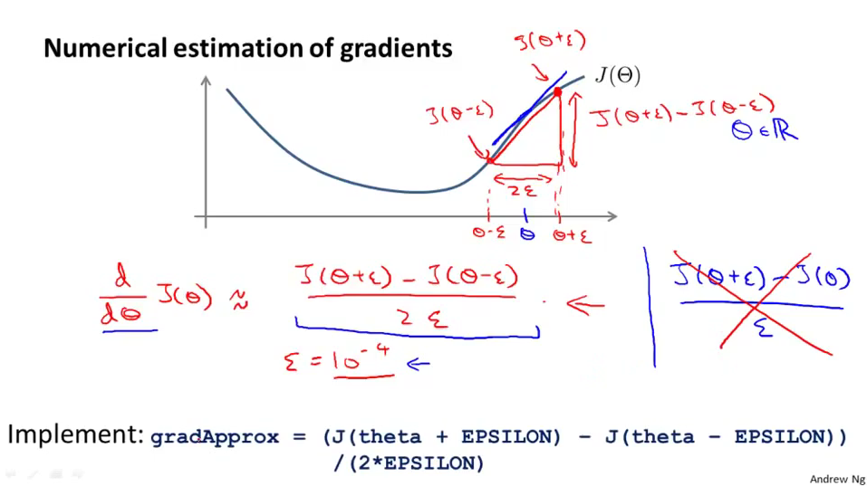
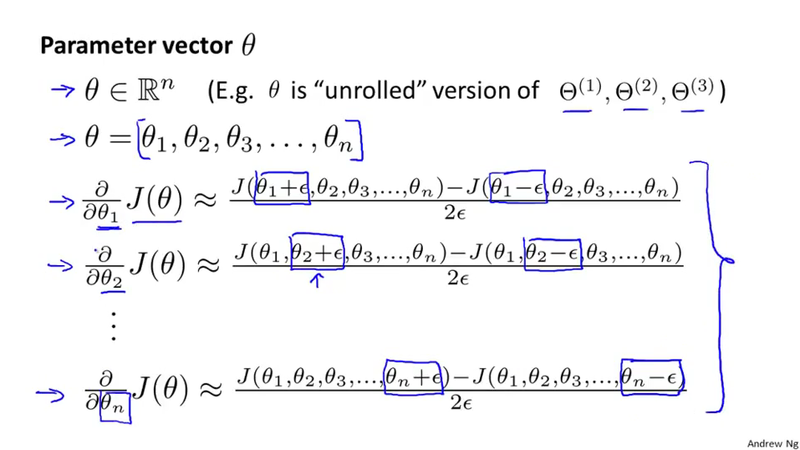
In Octave, we can implement this gradient checking as follows. We then want to check that gradApprox \approx deltaVector. Remove the gradient checking when you checking is done, otherwise the code is going to be very slow.
epsilon = 1e-4;
for i = 1:n,
  thetaPlus = theta;
  thetaPlus(i) += epsilon;
  thetaMinus = theta;
  thetaMinus(i) -= epsilon;
  gradApprox(i) = (J(thetaPlus) - J(thetaMinus))/(2*epsilon)
end;
Random Initialization
Initializing all theta weights to zero does not work with neural networks. When we back propagate, all nodes will update to the same value repeatedly.
Instead we can randomly initialize our weights: initialize each \Theta_{ij}^{(l)} to a random value between [-\epsilon, \epsilon].
In Octave, we can use the following code to generate the initial theta values.
#If the dimensions of Theta1 is 10x11, Theta2 is 10x11 and Theta3 is 1x11.

Theta1 = rand(10,11) * (2 * INIT_EPSILON) - INIT_EPSILON;
Theta2 = rand(10,11) * (2 * INIT_EPSILON) - INIT_EPSILON;
Theta3 = rand(1,11) * (2 * INIT_EPSILON) - INIT_EPSILON;
rand(x,y) will initialize a matrix of random real numbers between 0 and 1. (Note: this \epsilon is unrelated to the \epsilon from Gradient Checking)
Putting it Together
First, pick a network architecture; choose the layout of your neural network, including how many hidden units in each layer and how many layers total.
- Number of input units = dimension of features x^{(i)}
- Number of output units = number of classes
- Number of hidden units per layer = usually more the better (must balance with the cost of computation as it increases with more hidden units)
Defaults: 1 hidden layer. If more than 1 hidden layer, then the same number of units in every hidden layer.
Week 6 Advice for applying machine learning
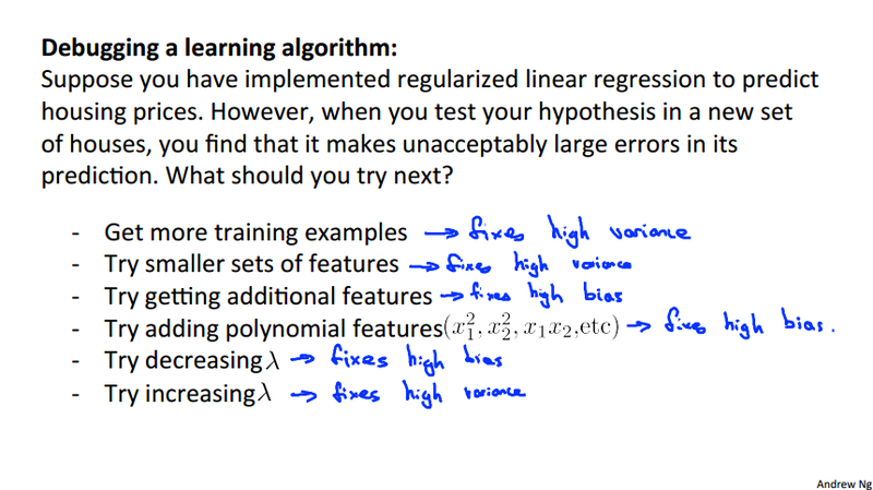
Deciding what to try next
- Get more training examples
- Try smaller sets\'of features
- Try getting additional features
- Try adding polynomial features
- Try decreasing \lambda
- Try increasing \lambda
Machine learning diagnostic
Diagnostic: A test that you can run to gain insight what is/isn\'t working with a learning algorithm, and gain guidance as to how best to improve its performance. It can take time to implement, but doing so can be a very good use of your time.
Evaluating a hypothesis
Diagnostic over-fitting by splitting the training set and test set
- Training set (70%)
- Test set (30%)
If the cost function J(\theta) calculated for training set is low, it is high for test set, over-fitting happens. This is apply to both logistic regression and linear regression.
Model selection and Train/Validation/Test sets
Normally we choose a model from a series of different degree of polynomial hypothesis, We choose the model that have the least cost for testing data. More specifically, we learned the parameter \theta^{(d)} (d is the degree of polynomial) from the training set and calculate the cost for the test dataset with the learned \theta. This is not the best practice for the reason that the hypothesis we selected has been fit to the test set. It is very likely the model will not fit new data very well.
We can improve the model selection by introduce the cross validation set. We divide our available data as
- Training set (60%)
- Cross validation set (20%)
- test set (20%)
We use the cross validation data to help us to select the model, and using the test data, which the model never see before to evaluate generalization error.
Warning
Avoid to use the test data to select the model (select the least cost model calculated on the test data set) and then report the generalization error using the test data.
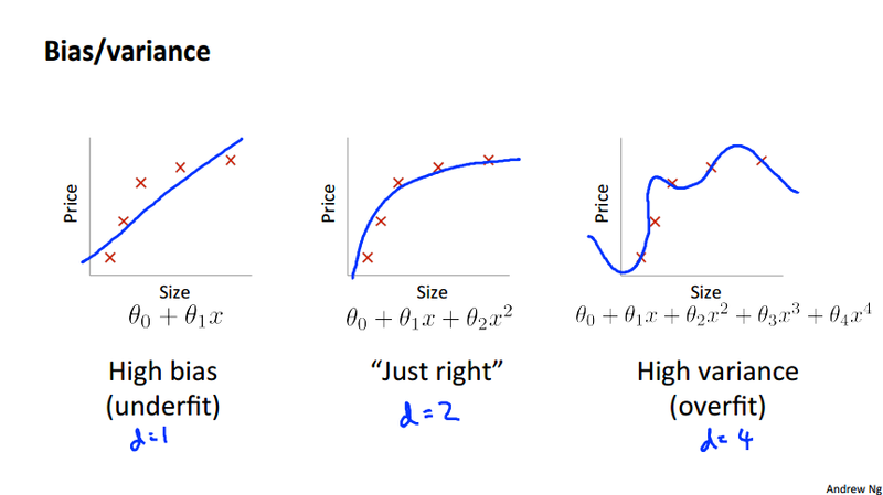
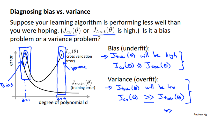
Diagnosing bias vs. variance
The important point to understand bias and variance is to understand how the cost for training data, cross validation data (or test data) changes.
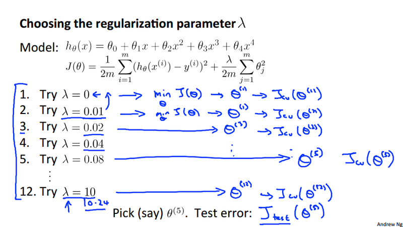
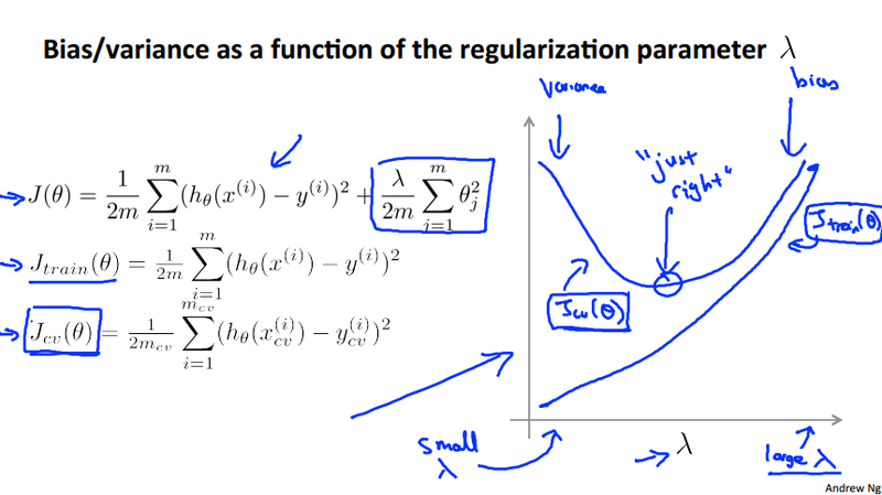
Regularization and bias/variance
The regularization parameter \lambda could play important role in selecting the best model to fit the data (both cross validation data and test data). This section will study how \lambda affect the cost function both for the training data and cross validation data.
Learning curve
This section mainly discuss how the sample size affect the cost function. There are two kinds of problem we face, high bias and high variance
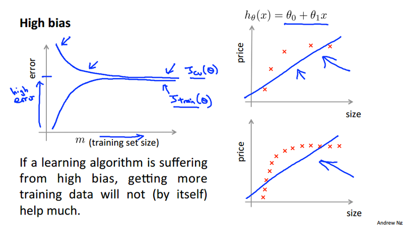
High bias
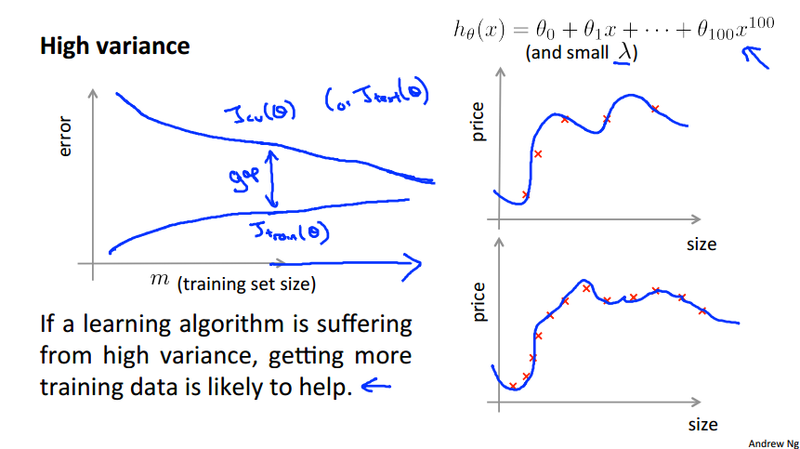
High variance
Deciding what to do next revisited
| bias/variance | underfitting/overfitting | regularization | to improve |
|---|---|---|---|
| High bias | underfitting | bigger lambda | more sample will not help much |
| High variance | overfitting (high polynomial) | smaller lambda | more sample will likely to help |
Prioritizing what to work on
Building a spam classifier
Error analysis
- Start simple algorithm, implement it and test it on cross-validation data.
- Plot learning curves to decide if more data, more features, etc. are like to help.
- Error analysis: Manually examine the examples (in cross validation set) that you algorithm make errors on. See if you spot any systematic trend in what type of examples it it making error on.
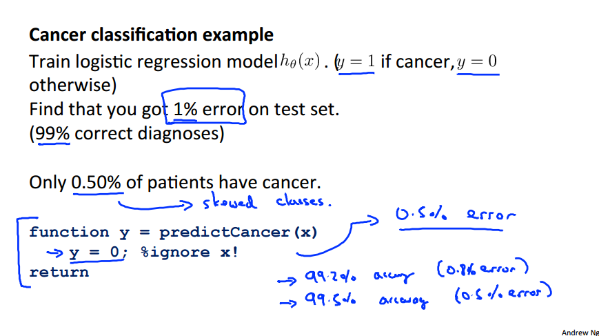
Error metrics for skewed classes
Problem arise in error analysis when only very small(less than 0.5%) negative samples possibly exist. Take the cancer classification as a example.
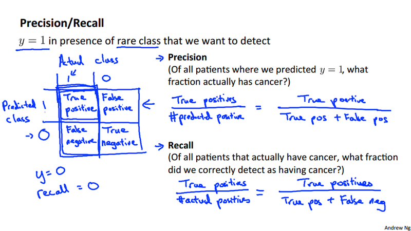
Precision and Recall
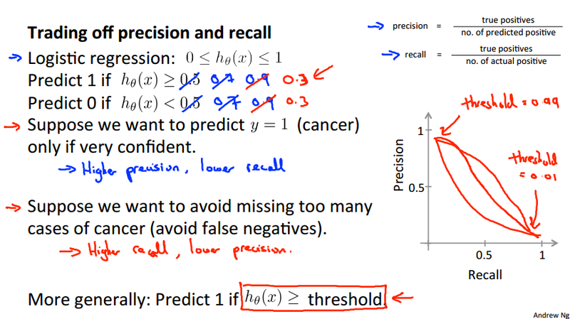
Trading off precision and recall
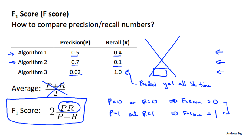
F score {#f_score}
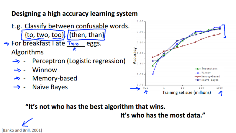
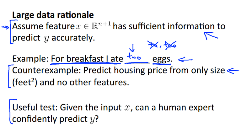
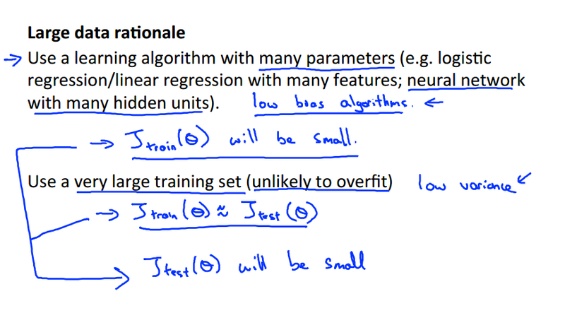
Data for machine learning
Week 7 Support Vector Machine
Optimization objective
SVM will be derived from logistic regression. There are not that much of logic, just following the derivation in the lecture. Let's first review the hypothesis of the logistic regress and its cost function:
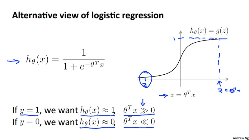
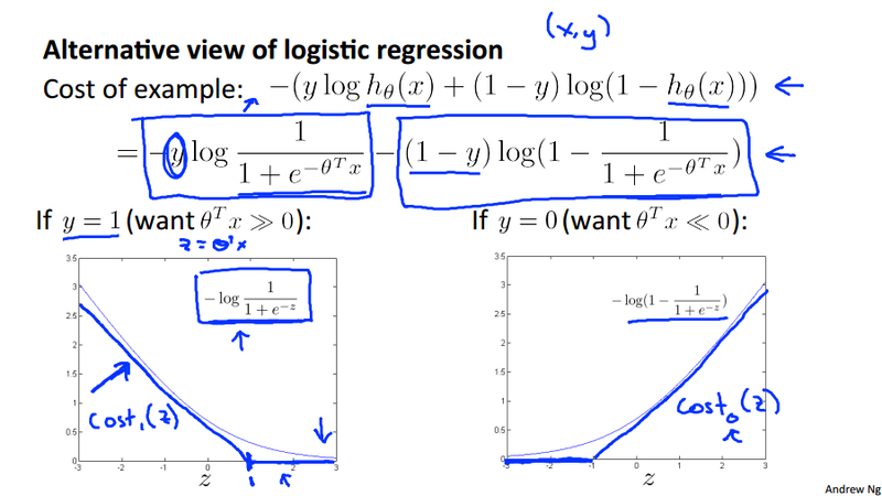
Notice in the second figure above, we define approximate functions cost_0(z) and cost_1(z). These functions will be used in the SVM cost function we will see next.
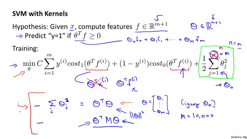
SVM cost function
Compare to logistic regression, SVM use a different parameters C. As in logistic regression, we use \lambda to control the trade off optimizing the first term and the second term in the objective function.
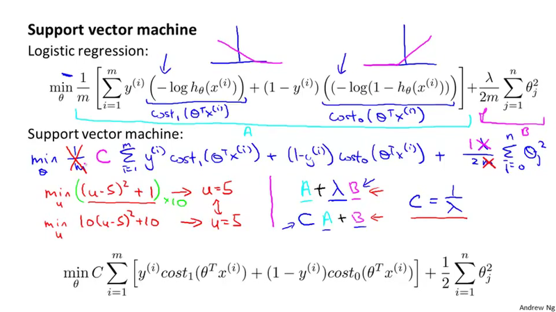
What's more, the SVM hypothesis doesn\'t give us a probability prediction, it give use either 1 or 0. Such as h_\theta = \begin{cases} 1 \qquad \text{if}\ \Theta^Tx \geq 0\\ 0 \qquad \text{otherwise} \end{cases}
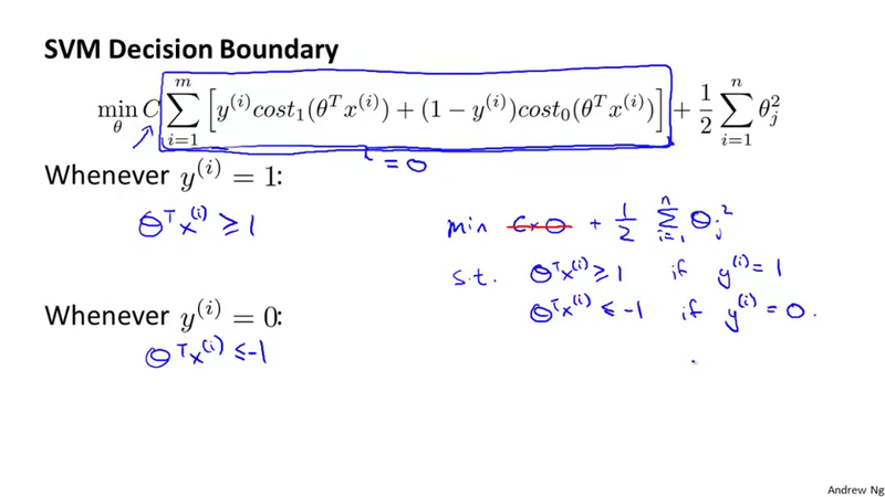
Large margin intuition
Suppose we make the parameter C very large, we want to make the first term in the summation approximate 0. We can derive the problem as a optimization problem subject to some condition. This optimization problem will lead us to discuss the decision boundary. when C is very large, the decision boundary will have a large margin, thus large margin classifier. Later we will see that using different kernel and parameters can control this margin.
Question
How the large margin classifier related to the optimization problem when C is very large?
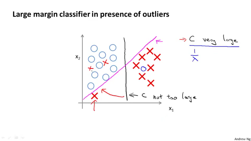
When C is very large, we have the magneto decision boundary, if C is not very large, we will have the black decision boundary, which is having the large margin properties.
Mathematics behind large margin classification
Using the vector inner product to transform the constrain from \theta^T x^{(i)} \geq 1 to p^{(i)}\Vert\theta \Vert \geq 1 for y^{(i)} = 1
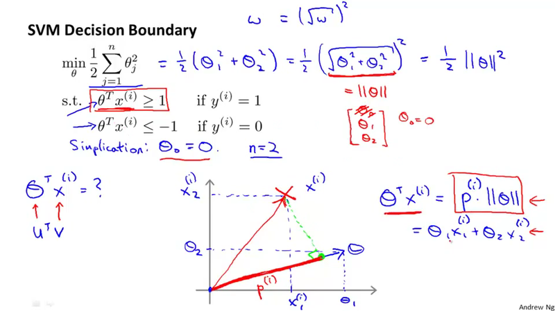
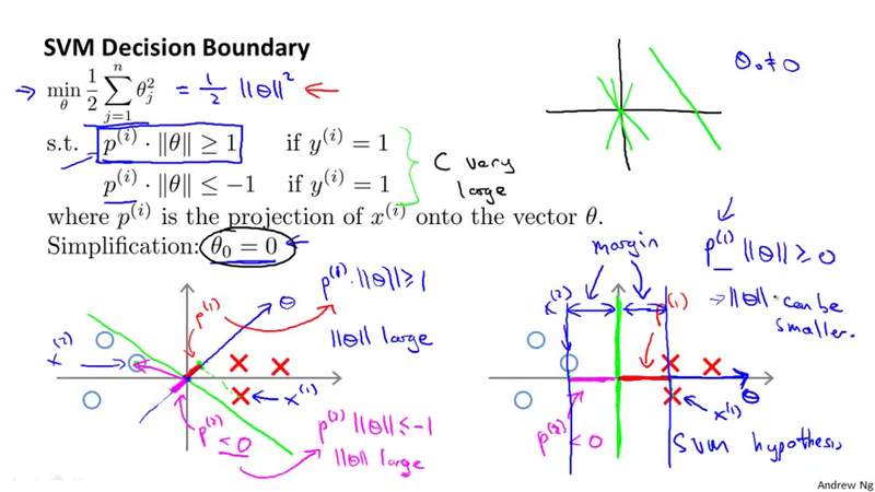
The point of this section is to discuss the mathematical insight why SVM choose the large margin decision boundary. (because, the large margin decision boundary will produce a larger p^{(i)}, thus a smaller \Vert\theta \Vert in the constrain of the optimization problem, so as to minimize the objective function \min_\theta \frac{1}{2} \sum_{j=1}^{n} \theta_j^2)
Kernel
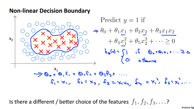
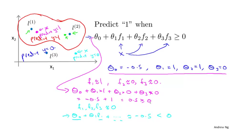
Non-linear decision boundary
Is there a different/better choice of the features f_1, f_2, f_3, \dots,
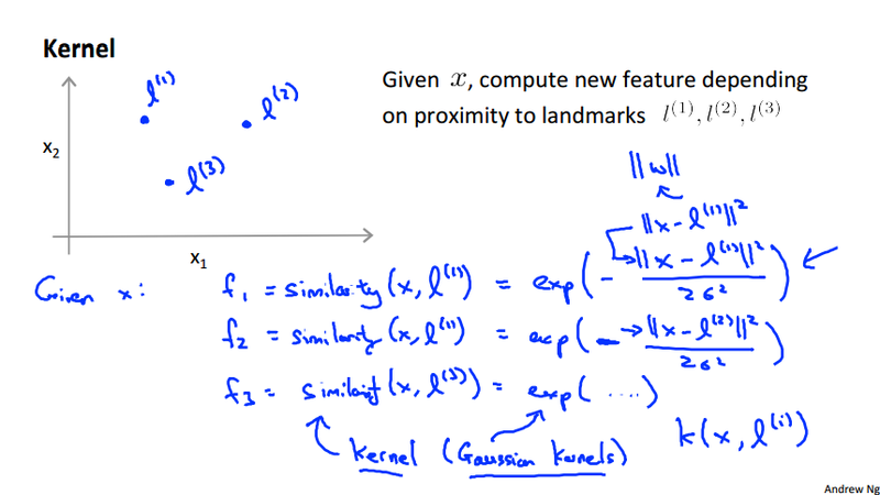
Landmarks
To respond the above question, we use the following way to generate the new features f_1, f_2, f_3, \dots,. Compare the similarity between the examples and the landmarks using a similarity function.
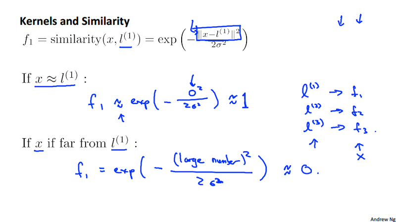
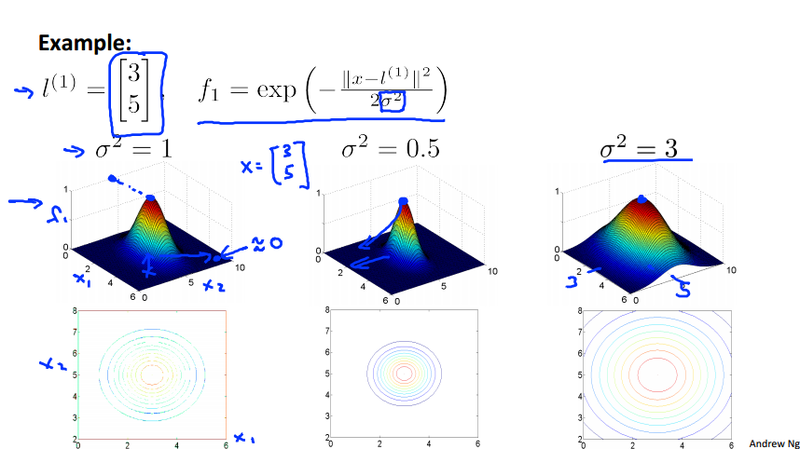
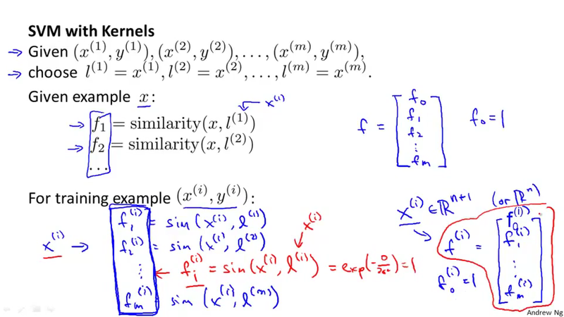
Gaussian kernel
We use the Guassian kernel k(x, \ell^{(i)}) = \exp(-\frac{\Vert x - \ell^{(i)}\Vert^2}{2\delta^2}) as the similarity function to generate the new feature.
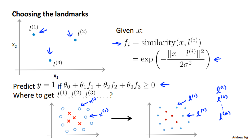
Choosing the landmarks
Naturally, we are going to choose the example itself as the landmark, thus we are able to transform the feature x^{(i)} to feature vector f^{(i)} for training example (x^{(i)}, y^{(i)}).
Using SVM
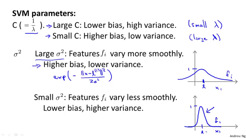
- Choice of parameter C.
- Choice of kernel (similarity function):
- No kernel ("linear Kernel")
- Gaussian kernel (need to choose \delta^2)
Because the similarity function is apply to each feature, we\'d better to perform feature scaling before using the Gaussian kernel. (take the house price features as an example, the areas and the number of rooms are not in the same scale.)
Note
Not all similarity functions similarity(x, \ell) make valid kernels. Need to satisfy technical condition called "Mercer's Theorem" to make sure SVM packagesl' optimizations run correctly, and do not diverge).
Many off-the-shelf kernels available:
- Polynomial kernel: k(X, \ell) = (X^T\ell + c)^{p}, such as k(x, \ell) = (X^T\ell + 1)^2.
- More esoteric: String kernel, chi-square kernel, histogram intersection kernel, ...
Note
Many SVM packages already have built-in multi-class classification functionality. Otherwise, we can use one-vs.-all method. Specifically, train K SVMs, one to distinguish y = i from the rest, for i = 1, 2, \dots, K, get \theta^{(1)}, \theta^{(2)}, \dots, \theta^{(K)}, pick class i with largest (\theta^{(i)})^Tx.
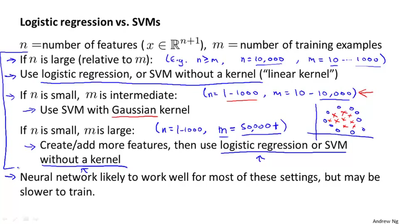
Logistic regression vs. SMVs
This section mainly discuss when to use logistic regression vs. SVM from the high level. I summarize the content of the slides in the table.
| n | m | logistic regression vs. SVMs |
|---|---|---|
| large (relative to mm) i.e. 10,000 | 10 - 1000 | use logistic regression, or SVM without a kerenl ("linear kernel") |
| small (i.e. 1-1000) | intermediate (10-10,000) | use SVM with Gaussian kernel |
| small (i.e. 1-1000) | large (50,000+) | create/add more features, then use logistic regression or SVM without a kernel |
Week 8 Unsupervised Algorithms
K-Means Algorithm
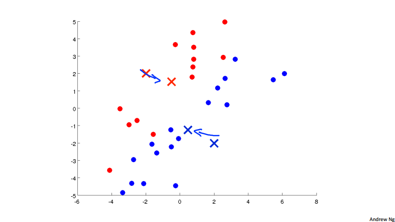
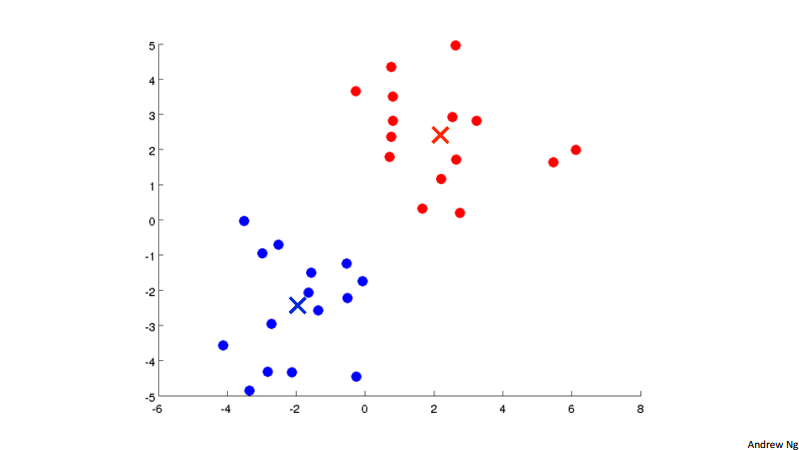
In the k-means clustering algorithm. We have input K (number of clusters) and traning set \{x^{(1)}, x^{(1)}, \dots, x^{(m)}\}, for each of the training example x^{(i)}\in \R^n. Note here we drop the x_0 = 1 convention. To visualize the algorithm, we have the following three picture.
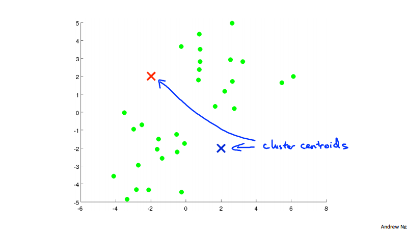
Concretely, the k-means algorithm is:
- Input: training set \! \{x^{(i)}\}_{i=1}^m, and number of clusters K.
- Algorith:
- Randomly initialize K cluster centroids \mu_1, \mu_1, \dots, \mu_K\in \R^n.
- Repeat:
- for i = 1 to m: // cluster assignment step
- c^{(i)} := index (from 1 to K) of cluster centroid closest to x^{(i)}
- for k = 1 to K: // move centroid step
- \mu_k := average (mean) of points assigned to cluster k
- for i = 1 to m: // cluster assignment step
- Until convergence
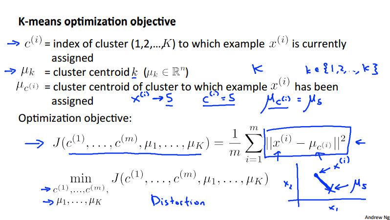
Optimization objective
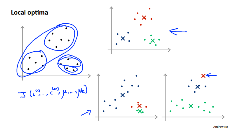
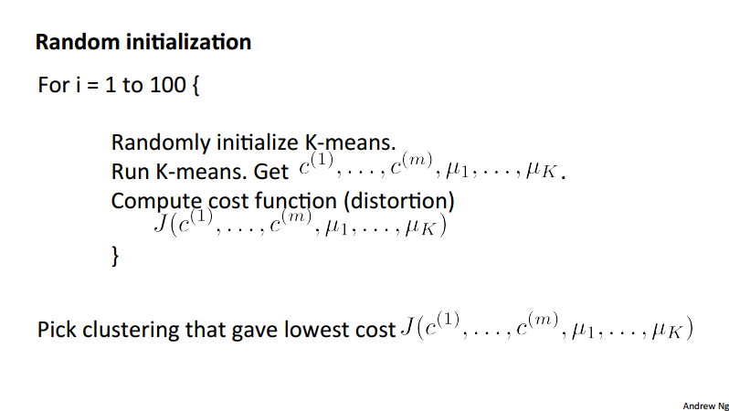
Random initialization
We can random initialize the centroid by randomly pick K training examples and set \mu_1, \dots, \mu_K equal to these K examples. Obviously, we should have K < m. However, some of the random initialization would lead the algorithm to achieve local optima, which is shown below in the pictures. To solve this problem, we can random initialize multiple times then to pick clustering that gave lowest cost J(c^{(1)}, \dots, c^{(m)}, \mu_1, \dots \mu_K).
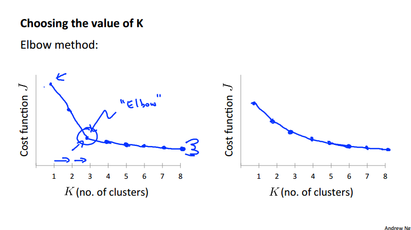
Choosing the K
It depends on the problem we are trying to solve. One straightforward problem is using a method called the Elbow method as the following picture. Secondly, the K value should be picked to maximize some practical utility function, for example, we cluster the size of different T-shirts, whether we want to have 3 sizes or 5 sizes is depends on the profitability.
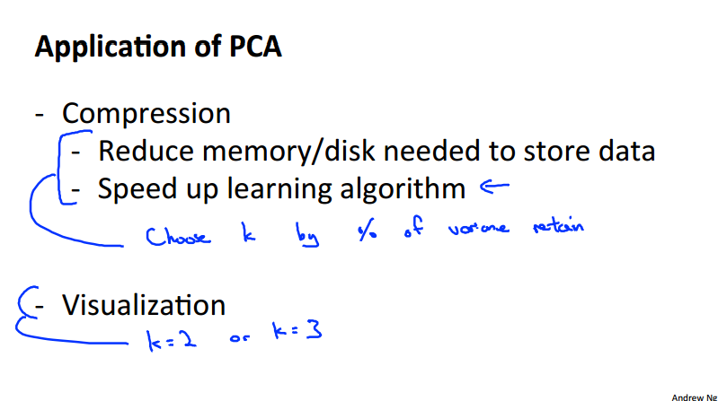
Dimensionality reduction
The two motivation of Dimensionality Reduction are:
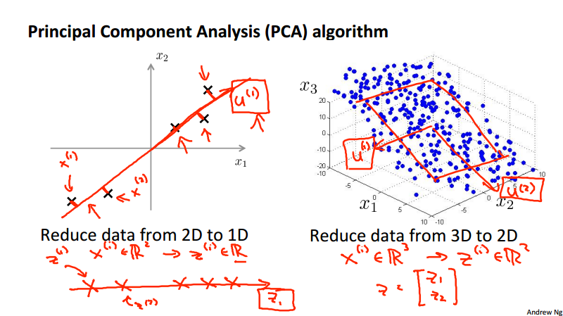
- Data compression, for example, reduce data from 2D to 1D.
- Visualization, we can reduce the high dimensionality data to 2 or 3 dimensions, and visualize them. For example, to visualize some complex economical data for different countries.
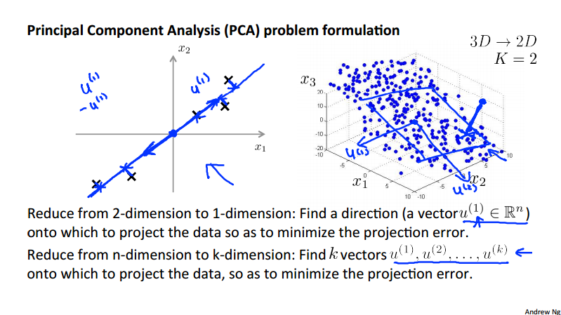
Principal Component Analysis (PCA)
To reduce from 2-dimension to 1-dimension: Find a direction (a vector u^{(1)}\in \R^n) onto which to project the data so as to minimize the projection error. To reduce from n-dimension to k-dimension: Find k direction vectors u^{(1)}, u^{(2)}, \dots, u^{(k)} onto which to project the data so as to minimize the projection error.
Note
Note the difference between PCA and linear regression.
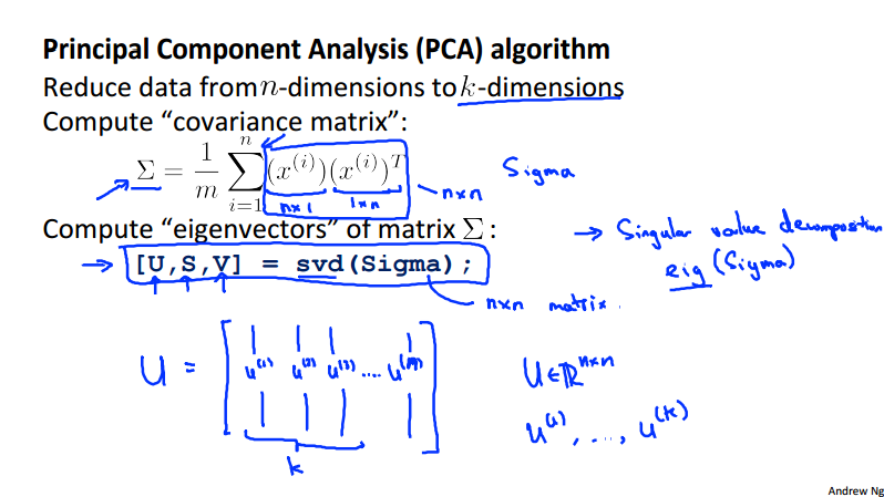
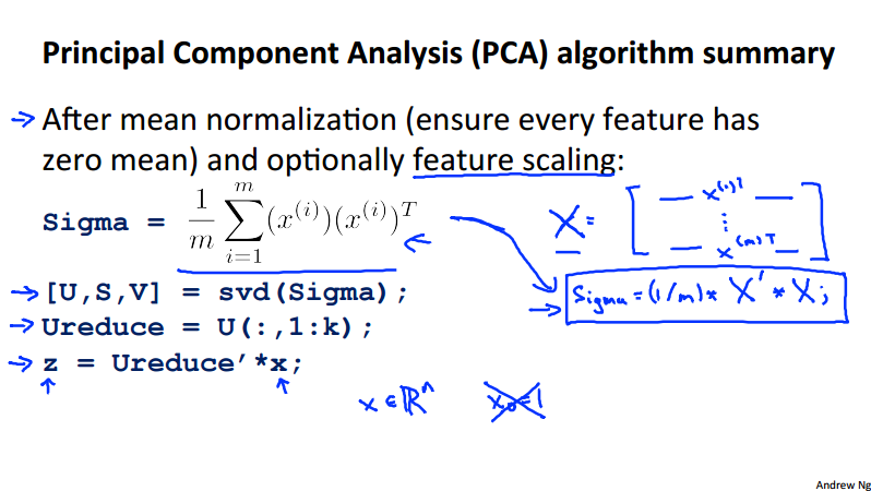
PCA algorithm
Before carry out the PCA, we\'d better to do some feature scaling/mean normalization. As in the slides below, the S_i could be the maximum/minimum value or other values such as variance \sigma.
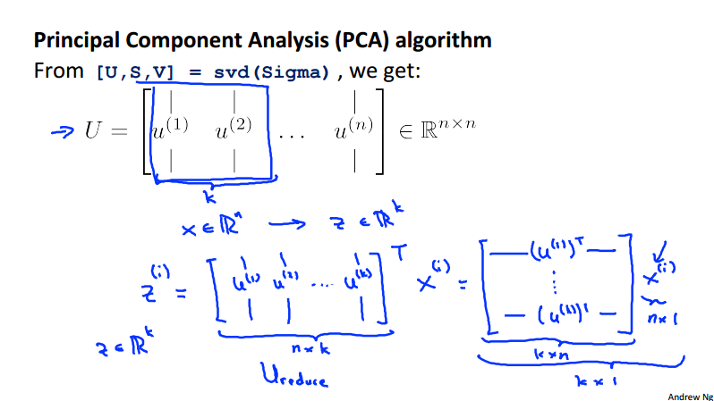
once the pre-proccessing steps are done we can run the following algorithm in Octave to implement PCA.
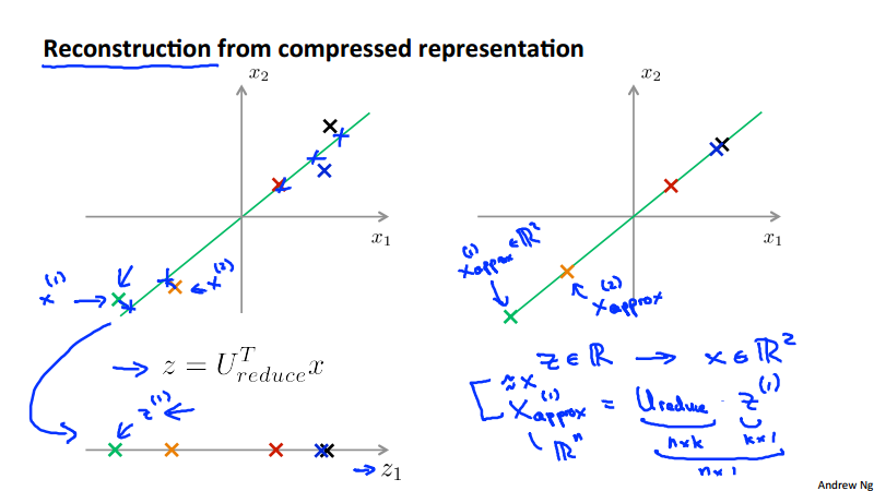
Reconstruction from PCA compressed data
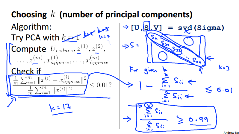
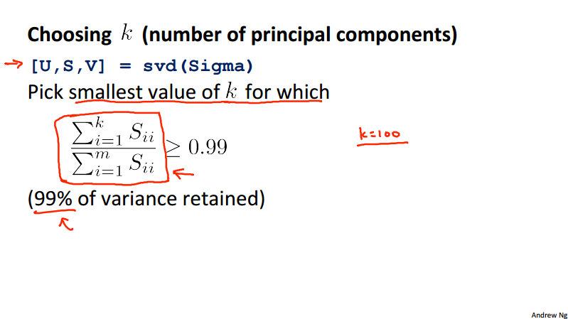
Choosing the number of principal components
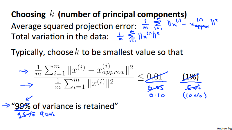
Two concepts we should define here:
Average squared projection error:
- \frac{1}{m}\sum_{i=1}^{m}\lVert x^{(i)} - x_{approx}^{(i)}\rVert^2
Total variation in the data:
- \frac{1}{m}\sum_{i=1}^{m}\lVert x^{(i)} \rVert^2
Typically, we choose k to be smallest value so that ration of the two quality should be less than 1%.
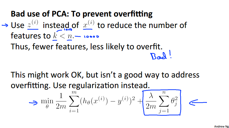
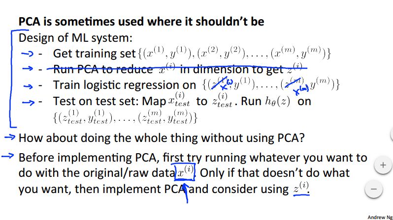
Advice for applying PCA
One important point should keep in mind when using PCA:
- don't try to use PCA to prevent overfitting, use regularization instead.
Week 9 Anomaly Detection
Anomaly Detection
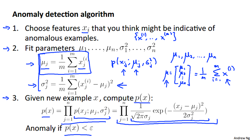
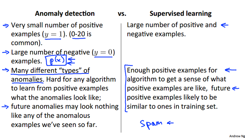
Given a model p(x), test on the example x^{(i)} to check whether we have p(x) < \epsilon. Generally, the anomaly detection system apply to the scenario that we don't have much anomaly example, such as a dataset about aircraft engines.
In this particular lecture, the p(x) is multivariate Gaussian distribution. The algorithm is to find the parameter \mu and \sigma^2. Once we fit the data with a multivariate Gaussian distribution, we are able to obtain a probability value, which can be use to detect the anomaly by select a probability threshold \epsilon.
Here is the anomaly detection algorithm:
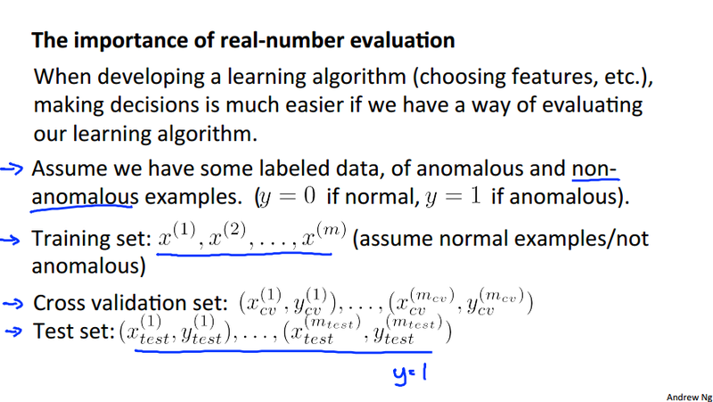
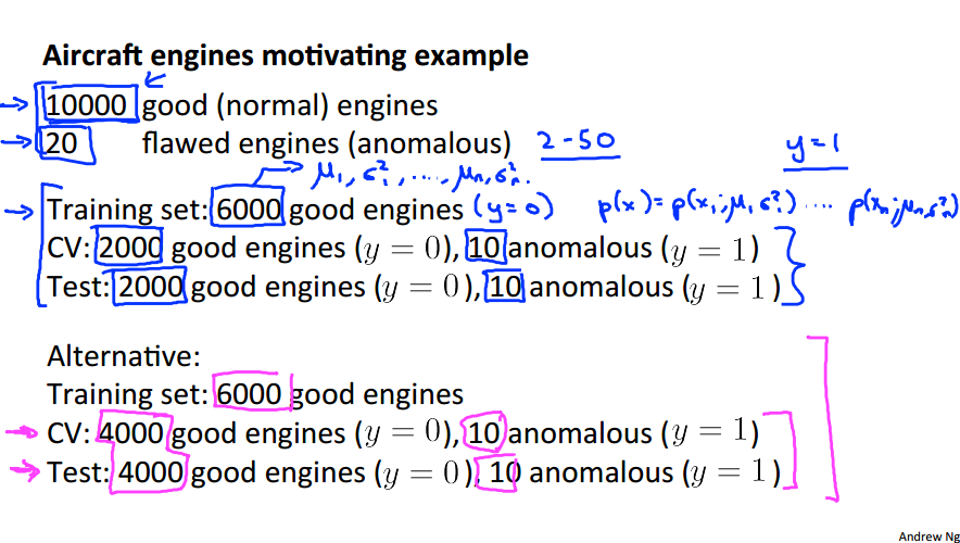
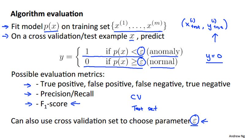
Developing and evaluating
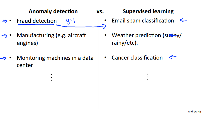
Anomaly detection vs. supervised learning
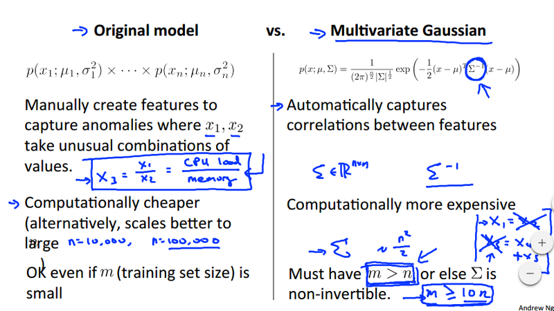
Multivariate Gaussian distribution
There are plots of different multivariate Gaussian distributions with different mean and covariance matrix. It intuitively show how changes in the mean and covariance matrix can change the shape of the plot of the distribution. It also compared the original model (multiple single variate Gaussian distribution) to multivariate Gaussian distribution. Generally, if we have multiple features, we tend to use multivariate Gaussian distribution to fit the data, even thought the original model is more computationally cheaper.
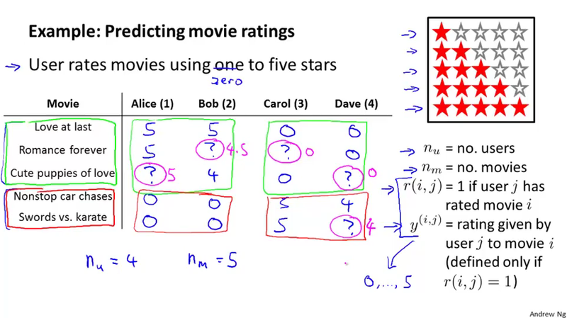
Predicting movie ratings
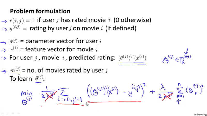
Problem formulation
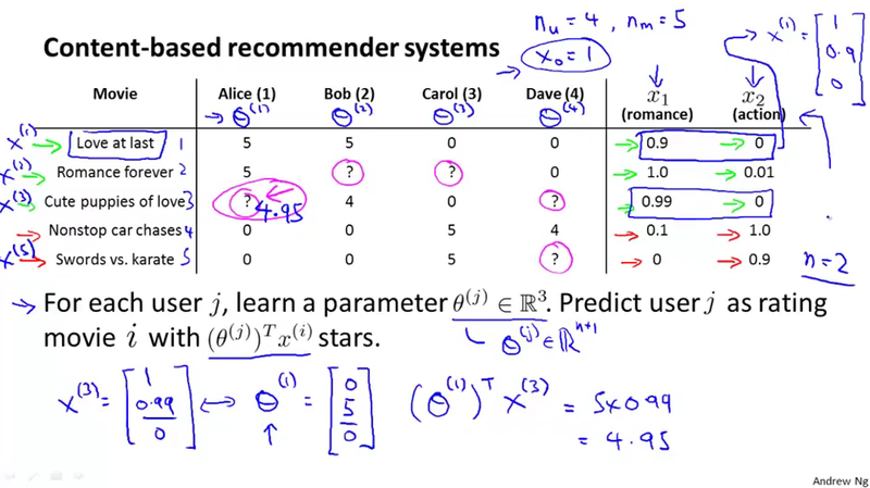
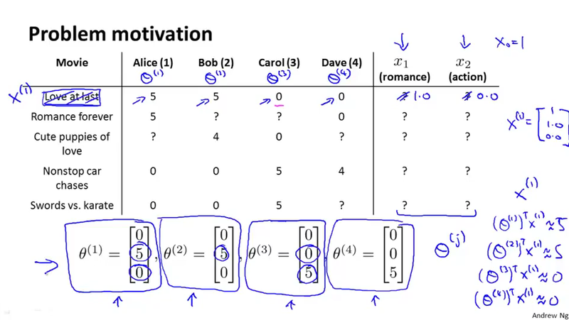
Content based recommendations
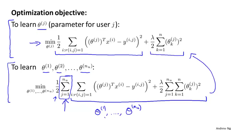
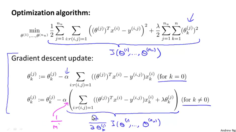
Suppose we have a feature vector for each of the movie, combining with the rating values, we can solve the minimization problem to get \theta^{(j)}, which is the parameter vector of user j. With this parameter vector, we can predicting the rating of the movie by (\theta^{(j)})^T x^{(i)}.
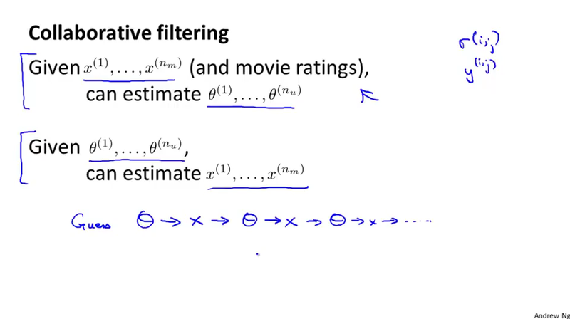
Collaborate filtering
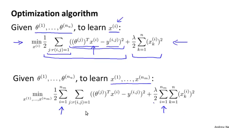
In collaborate filtering, we don\'t have the feature, we only have the parameter vector \theta^{(j)} for user j. We can solve a optimization problem in regarding to the feature vector x^{(i)} through the rating values.
What interesting about this if we don\'t have the initial \theta^{(j)}, we can generate a small random value of \theta^{(j)}, and repetitively to get the feature vector x^{(i)}. As later we can say, we can solve a optimization problem with regarding to both \theta^{(j)} and x^{(i)} all at once. See the slides for details.
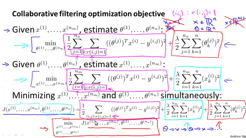
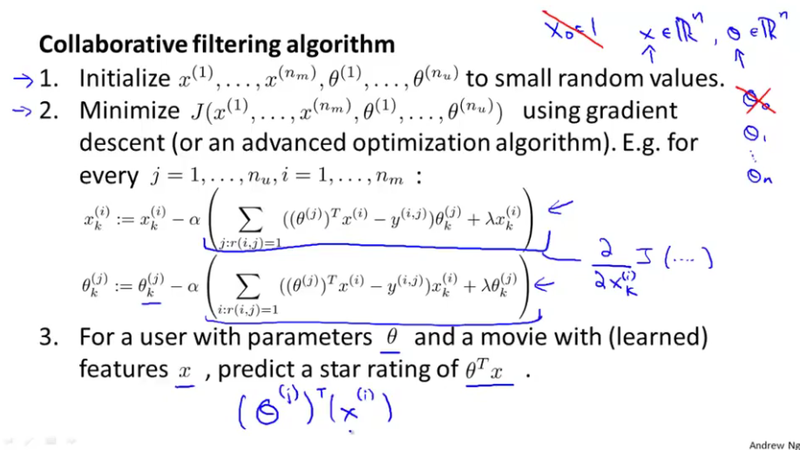
Collaborative filtering algorithm
As discussed above, in practice, we solve the optimization problem respect to both \theta^{(j)} and x^{(i)}. See the slides for the optimization problem we are trying to solve, and the gradient descent algorithm to solve it.